[I7R8]

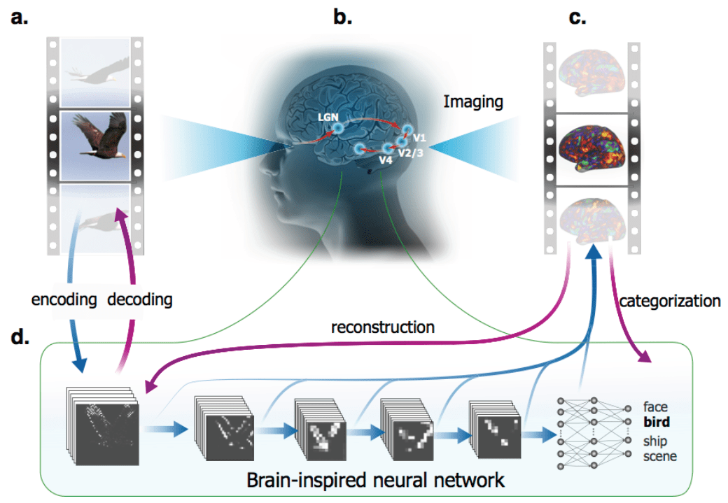
Wen, Shi, Zhang, Lu & Liu (pp2016) used a deep feedforward convolutional neural network (CNN) as an encoding model for fMRI data acquired while human subjects viewed movies. Previous studies (Yamins et al. 2014; Khaligh-Razavi & Kriegeskorte 2014; Güçlü & van Gerven 2015; Eickenberg et al. 2016) found that deep convolutional networks provide good models of the representation of natural images in higher ventral-stream areas. Wen et al.’s deep-net prediction of fMRI responses during movie viewing extends these findings to dynamic viewing conditions (see also Eickenberg et al. 2016 for initial deep net analyses of movie fMRI data).

The deep net was similar to AlexNet in architecture and had been trained to classify static images. The model processed each frame separately through its purely feedforward hierarchy and had no mechanism for recognising visual motion and more complex visual dynamics. Nevertheless, it did quite well at explaining visual fMRI responses during movie viewing. This is perhaps expected based on previous studies of fMRI responses during movie viewing (Hasson et al. 2001), which showed that category-selective regions respond as expected during movie viewing, when their preferred categories are present in the scene.

The authors conduct a series of original and well-motivated analyses, including decoding and deconvolution, to explore the degree to which the deep network captures the dynamic representations at multiple levels. Overall, this is a technically excellent study providing further evidence that deep feedforward neural networks constitute good models of ventral-stream responses, with layers roughly corresponding to stages of processing along the ventral stream.

Results are largely consistent with expectations from previous studies, but the study is a good contribution because it replicates and generalises earlier findings. We are wondering whether more novel insights could be gained by empirically demonstrating the limitations of the model (feedforward, no motion or dynamic perception). This could be achieved by showing that the model does not explain all the explainable variance in the data and where in the brain the deep convolutional feedforward model falls short. Eventually, the field will need to compare multiple deep neural network models (including feedword models that take multiple frames as input, and recurrent models that can dynamically compress the recent stimulus history as biological visual systems probably do).

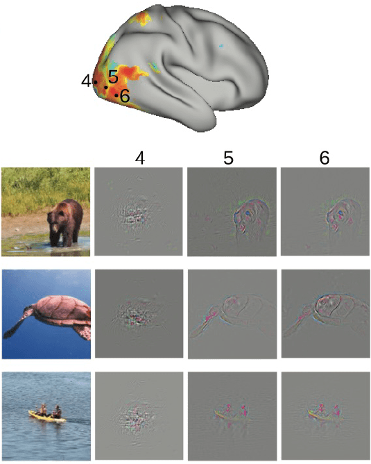
Figure: Visualising the image features that drive fMRI voxel responses in the context of particular images. Using the deconvolutional visualisation technique of Zeiler & Fergus on voxel encoding models (deep convolutional network + ridge regression), enables the authors to visualise to what extent adjusting pixels of a particular image (photos on the left) would change the encoding model’s prediction about voxel activity. Results shown here are for three voxels at different stages of the hierarchy. Voxel 4 has a localised central small receptive  field. Voxels 5 and 6 have larger receptive fields.

 

Main findings

Voxel-to-units matching characterises cortical responses

The paper demonstrates the functional alignment between the visual cortex and the CNN using a simple and effective method: each voxel’s time course during movie viewing is correlated with the output of each CNN unit when exposed to the frames of the movie (after convolution with a kernel to account for the delay and smoothness of the hemodynamic response). The highest-correlating units are then considered as matches. Note that this simple matching of each voxel to a set of units is easier to interpret than fitting a linear encoding model, which would have continuous weights spread over a large number of units. A disadvantage of simple voxel-to-unit matching might be that it doesn’t account for the averaging in fMRI voxels.

• For early visual areas, the authors estimate population receptive field properties of each voxel by averaging the matching CNN units’ receptive field properties. The authors restrict this analysis to layer 1 of the CNN and recover plausible retinotopic maps from the movie responses with this method.
• Across the stages of the visual hierarchy, the authors label each voxel with the CNN layer that best explains it (see also Güçlü & van Gerven 2015). Here the authors assigned each voxel to the CNN layer containing the unit that achieved the maximum correlation with the voxel response. Consistent with the previous studies, this reveals a largely monotonic correspondence between the stages of the visual hierarchy and the layers of the CNN.

 

The CNN layer-8 face detector unit is correlated with the fusiform face area

The authors correlated voxels with an output unit trained to detect faces. The resulting univariate brain map highlights face-selective regions, including the fusiform face area (FFA). We already knew that FFA responds to faces, and does so during natural vision (movies; e.g. work by Hasson et al.). We also know that CNNs can recognise faces. Putting these together, CNNs must be able to predict responses of the FFA to some degree. Indeed previous studies have already explicitly shown that CNNs explain variance in FFA (Khaligh-Razavi et al. 2014, Fig. S3b; Eickenberg et al. 2016). Being able to detect faces is necessary for a computational account of FFA, but it is not sufficient. We are left wondering whether the model can explain the FFA profile of activation within faces and within inanimate images (Mur et al. 2012) or the representational geometry within those two categories.

 

Encoding models linearly combining CNN units can predict voxel responses to novel movie segments

The authors used CNN units as nonlinear image features of ridge regression models of voxel responses. They logarithmically transformed the CNN outputs to model a saturating response that better matches the distribution of fMRI response amplitudes across images. They convolved the unit responses to movie frames with a hemodynamic response function to model the smoothness and delay of fMRI responses. As in previous studies, these models were tested for generalisation to novel stimuli (different movie segments here). They explained significant variance across large swaths of visual cortex.

 

FFA encoding model prefers face images

The authors attempted to visualise the preferences of the FFA by presenting 20,400 images from the same 15 categories to the encoding model. These images were not used for training the deep net and were not part of the fMRI experiments used to train the encoding model. Of the 1,000 (out of 20,400) images, for which the FFA voxel’s encoding model predicted the greatest response, 90.4% were faces.

The authors then averaged the images most strongly driving the FFA encoding model. They state: “Strikingly, the average visualization showed a blurred but discernable picture of a human face (Fig. 3.c, middle). For the first time, this result provides the direct visualization of the highly face-selective functional representation at FFA.”

This result is not particularly compelling and invites incorrect interpretations. It reflects the known fact that FFA responds to faces (Kanwisher et al. 1997) and the central/frontal-view bias for faces in the image set used to make the visualisation. Visualising the FFA response as an image template misses the point of a deep hierarchy of nonlinear transformation: If an image template could characterise the response of FFA, multiple nonlinear transformations would not be needed.

To test for the necessity of multiple nonlinear stages, the encoding model could be replaced by a template matcher. More generally, model compression could be used to attempt to explain the FFA response with a shallower model. This might yield deeper insights into the computations underlying FFA responses.

 

Deep convolutional encoding models can be combined with deconvolutional inversion to visualise what image features drive individual voxels

The authors use the deconvolutional visualisation technique of Zeiler & Fergus on voxel encoding models (deep convolutional network + ridge regression). This is a good idea. It enables the authors to visualise, for a particular image, what pixels most strongly affect the encoding model’s prediction of voxel activity. Again, a single template image cannot characterise a deep convolutional encoding model. However, looking at the encoding model’s gradient in image space in the context of many probe images might help us understand the model’s computation.

 

Images and semantic categories can be decoded not only within, but also between subjects

The authors analyse to what extent encoding and decoding models fitted with one subject’s data generalise to other subjects. It’s good to have these analyses in the paper because they give us a more quantitative sense of the degree to which the anatomical intersubject alignment succeeds at matching up functionally similar responses. As expected, within-subject encoding and decoding predictions are more accurate, but generalisation across subjects does work somewhat.

 

Decoding models can reconstruct natural movie stimuli and reveal semantic categories

The authors estimated multivariate regression models to predict time-varying feature maps of CNN layer 1 based on distributed cortical fMRI signals. Training was performed using an L1 (sparsity encouraging) penalty on the weights and random dropping out of a subset of the voxels during training with stochastic gradient descent. The layer-1 representation was then converted back to an image. As expected from previous studies (Thirion et al., Nishimoto et al., Miyawaki et al.) this works to some extent, highlighting regions of the image with high edge energy. The authors also decode semantic categories, which works quite well (again, not unexpectedly).

 

Strengths

• tests a task-performing neurobiologically plausible (though abstract) deep neural network model
• replicates previous findings on deep convolutional nets as models of fMRI visual responses and generalises these findings to movie viewing
• analyses technically excellent in many respects
• analyses are comprehensive and well motivated
• brings the deconvolutional technique of for visualization of the model unit preferences (as gradient in image space in the context of particular preferred images) into the analysis of brain data
• high-quality figures
• well written

 

Weaknesses

• The authors follow the widespread approach of looking to confirm what the field already believes. The rationale of this approach could be described as follows: “Here’s a really cool and novel demonstration of what you already believe.” It is as though we are afraid to learn something new or do not trust our methods unless they confirm current opinion. If our methods are sound, we should be able to apply them to questions whose answers we don’t know yet. As a result, the analyses here largely confirm what we know (or think we know) rather than providing surprising or contradictory new leads.
• Some of the analyses shown are affected by selection bias. This is a widespread problem in systems neuroscience (Kriegeskorte et al. 2009). While the authors are certainly aware of the related challenges of overfitting, circularity, and selection bias (using separate training and test sets for both deep net training, and the fitting of encoding models), selective presentation of results in Figs. 2d, 3a, 7 might be misleading. It’s important to note that this problematic practice is widespread, motivated by a rationale that could be stated as follows: “Let me show what you already believe in a beautiful graph based on data selected to conform with what you believe and therefore biased (to an unknown degree) to confirm your belief.”

 

Points the authors may wish to address in revision

Selection bias

State clearly what data and criteria have been used to select voxels and ROIs whose results are shown (Figs. 2d, 3a, 3c, 7). Use independent data sets (1) for selection and ROI definition and (2) for estimating and plotting effects in the ROIs.

 

Inference must account for serial autocorrelation of fMRI time courses

Time points in fMRI are highly dependent, so cannot be considered exchangeable under H0. You could use prewhitening (e.g. the Cochrane-Orcutt method) or simulate a realistic null distribution by block permutation. Temporal block permutation could use long blocks and just enough of them to have a sufficient number of permutations. Some contexts where this applies are as follows:

• “The significance of the cross correlation was assessed by calculating the p-value with the degree of freedom equal to the number of time points minus 2 (DOF=238, p<0.001, Bonferroni correction for the number of voxels).”

• “The significance of the cross correlation was assessed by calculating the p-value with the degree of freedom equal to the number of time points minus 2 (DOF=238 with Bonferroni correction to account for the number of voxels and p<0.001).”

• “To test the statistical significance of the average prediction accuracy, we performed a permutation test. From the fMRI-estimated feature maps, a large set of permuted feature maps were created by randomly and temporally shuffling the estimated feature maps for 10000 times.”
  The shuffled entities should not be single time points.

• “For example, a ‘face’ neuron in the CNN was significantly correlated with the fusiform face area (FFA) (r=0.25±0.057, p<0.01, corrected) (Fig. 2.d, right).” Does this take serial autocorrelation into account?

 

Analyse where the deep convolutional net falls short

It would be great to visualise the ways the deep convolutional encoding model falls short.

• To what extent can the replicable movie-responses in higher parietal, temporal and frontal cortices that appear in Fig. 2a be explained by the deep net? What layers best explain them?
• In addition to the whole-brain cortical surface map of where the deep net explains significant variance, it would be good to see where it explains significantly less variance than another measurement for the same subject and the same movie segment. This would reveal where in the brain the deep net fails to explain all explainable variance.
• It would also be good to show what aspects of visual responses the deep net misses in regions where it performs well overall. One way to do this would be to compare the fMRI-based image reconstruction to an image reconstruction obtained with the same method from the encoding-model-predicted fMRI responses. We might expect, for example, that the encoding model misses the attentional mechanisms of the brain. The reconstructions from the encoding model prediction might therefore reflect the edge energy in the image, equally representing foreground object and background scene, whereas the fMRI reconstruction reflects attentional selection of the foreground object.

 

Deconvolution cannot invert a deep convolutional feedforward network

Several passages in the paper currently suggest that deconvolution exactly inverts the convolutional feedforward processing, for example:

• “It is worth noting that nonlinear features coded in the CNN were not isolated functions, but connected through hierarchical networks that are fully computable either bottom-up or top-down.”
• “In addition, the model is fully observable and computable both forward and backward (Zeiler and Fergus, 2014), such that the extracted features can be transformed, either top-down or bottom-up, to visualize their internal representations, to reconstruct the visual input, as well as to deduce its semantic categorization.”

However, rectified linear units and max-pooling are noninvertible, image-dependent switches and “transpose as inverse” only provide approximations, and many dimensions are intentionally discarded across stages of the feedforward hierarchy. Please clarify these approximations and how they relate to (a) the goal of reconstruction of the image and (b) the goal to visualise the image features driving particular model responses.

 

Open science

Will data and code be available for other researchers to build on the findings?

 

Image reconstruction with error-flow from all layers

Reconstruction of natural movie stimuli is performed based on the decoding from fMRI of the 1st layer of the CNN only. Higher layers of the CNN should be better decodable from higher cortical regions. The ideal reconstruction would simultaneously decode all layers of the CNN from all cortical regions, using this information as a joint constraint for image reconstruction. Image reconstruction could rely on backpropagation down to the image input, with error flow from all layers of the CNN.

fMRI-like preprocessing of the CNN outputs

The authors take the logarithm of CNN outputs and convolve with an HRF model kernel peaking at 4 s latency. It would be good to know how this reasonable approach performs in comparison to other approaches, e.g. leaving out the logarithmic transform and/or estimating the HRF and its peak latency for each voxel (e.g. Pedregosa et al. pp2014).

 

Motivation for different weight priors implicit to regularisation in encoding and decoding

In the encoding models, the weight regularizer is an L2 penalty (ridge regression), whereas in the decoding models it is an L1 penalty (LASSO).

• What’s the motivation for these choices?

• Were both approaches tried for both encoding and decoding? If results were different, what would be the implications?

• What is the motivation for dropout (another approach to regularisation) in fitting the decoders? Is it to prevent informative voxels to be pushed down because the L1 penalty encourages sparsity?

 

Language

There are some typos and minor grammatical errors (e.g. “in details” -> “in detail”).

 

– Nikolaus Kriegeskorte & Johannes Mehrer