What’s the best measure of representational dissimilarity?

[I3R3]

Bobadilla-Suarez, Ahlheim, Mehrotra, Panos, & Love (pp2018) set out to shed some light on the best choice of similarity measure for analyzing distributed brain representations. They take an empirical approach, starting with the assumption that a good measure of neural similarity should reflect the degree to which an optimal decoder confuses two stimuli.

Decoding indeed provides a useful perspective for thinking about representational dissimilarities. Defining decoders helps us consider explicitly how other brain regions might read out a representation, and to base our analyses of brain activity on reasonable assumptions.

Using two different data sets, the authors report that Euclidean and Mahalanobis distances, respectively, are most highly correlated (Spearman correlation across pairs of stimuli) with decoding accuracy. They conclude that this suggests that Euclidean and Mahalanobis distances are preferable to the popular Pearson correlation distance as a choice of representational dissimilarity measure.

Decoding analyses provide an attractive approach to the assessment of representational dissimilarity for two reasons:

  • Decoders can help us test whether particular information is present in a format that could be directly read out by a downstream neuron. This requires the decoder to be plausibly implementable by a single neuron, which holds for linear readout (if we assume that the readout neuron can see a sufficient portion of the code). While this provides a good motivation for linear decoding analyses, we need to be mindful of a few caveats: Single neurons might also be capable of various forms of nonlinear readout. Moreover, neurons might have access to a different portion of the neuronal information than is used in a particular decoding analysis. For example, readout neurons might have access to more information about the neuronal responses than we were able to measure (e.g. with fMRI, where each voxel indirectly reflects the activity of tens or hundreds of thousands of neurons; or with cell recordings, where we can often sample only tens or hundreds of neurons from a population of millions). Conversely, our decoder might have access to a larger neuronal population than any single readout neuron (e.g. to all of V1 or some other large region of interest).
  • Decoding accuracy can be assessed with an independent test set. This removes overfitting bias of the estimate of discriminability and enables us to assess whether two activity patterns really differ without relying on assumptions (such as Gaussian noise) for the validity of this inference.

This suggests using decoding directly to measure representational dissimilarity. For example, we could use decoding accuracy as a measure of dissimilarity (e.g. Carlson et al. 2013, Cichy et al. 2015). The paper’s rationale to evaluate different dissimilarity measures by comparison to decoding accuracy therefore does not make sense to me. If decoding accuracy is to be considered the gold standard, then why not use that gold standard itself, rather than a distinct dissimilarity measure that serves as a stand in?

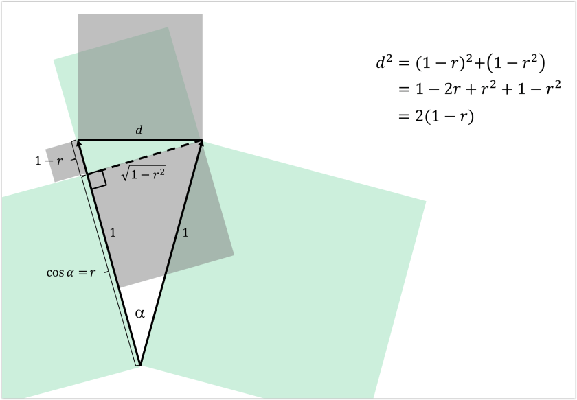
In fact the motivation for using Pearson correlation distance for comparing brain-activity patterns is not to emulate decoding accuracy, but to describe to what extent two experimental conditions push the baseline activity pattern in different directions in multivariate response space: The correlation distance is 1 minus the cosine of the angle the two patterns span (after the regional-mean activation has been subtracted out from each).

Interestingly, the correlation distance is proportional to the squared Euclidean distance between the normalized patterns (where each pattern has been separately normalized by first subtracting the mean from each value and then scaling the norm to 1; see Fig. 1, below and Walther et al. 2016). So in comparing the Euclidean distance to correlation distance, the question becomes whether those normalizations (and the squaring) are desirable.

correlation distance is normalized euclidean squared
Figure 1: The correlation distance (1-r, where r is the Pearson correlation coefficient) is proportional to the squared Euclidean distance d2 when each pattern has been separately normalized by first subtracting the mean from each value and then scaling the norm to 1. See slides for the First Cambridge Representational Similarity Analysis Workshop (http://www.mrc-cbu.cam.ac.uk/rsa2015/rsa2015media/) and Nili et al. (2014).

One motivation for removing the mean is to make the pattern analysis more complementary to the regional-mean activation analysis, which many researchers standardly also perform. Note that this motivation is at odds with the desire to best emulate decoding results because most decoders, by default, will exploit regional-mean activation differences as well as fine-grained pattern differences.

The finding that Euclidean and Mahalanobis distances better predicted decoding accuracies here than correlation distance, could have either or both of the following causes:

  • Correlation distance normalizes out to the regional-mean component. On the one hand, regional-mean effects are large and will often contribute to successful decoding. On the other hand, removing the regional-mean is a very ineffective way to remove overall-activation effects (especially different voxels respond with different gains). Removing the regional mean, therefore, may hardly affect the accuracy of a linear decoder (as shown for a particular data set in Misaki et al. 2010).
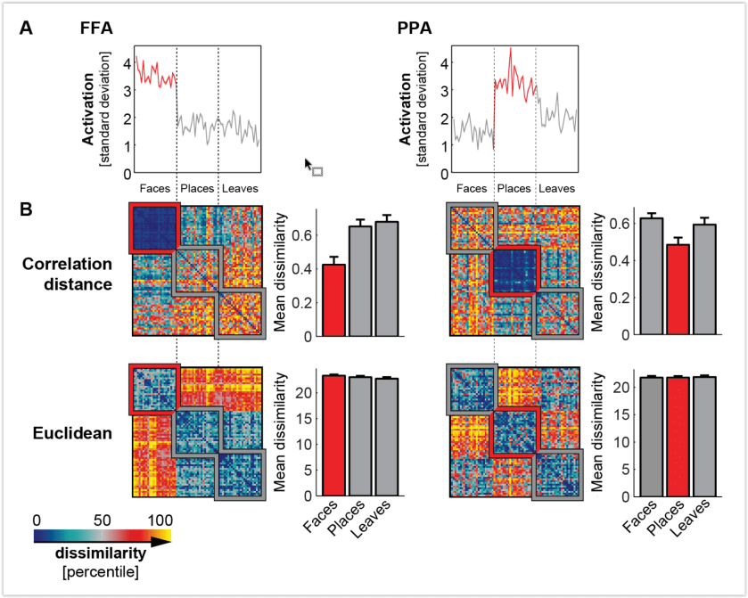
  • Correlation distance normalizes out the pattern variance across voxels. The divisive normalization of the variance around the mean has an undesirable effect: Two experimental conditions that do not drive a response and therefore have uncorrelated patterns (noise only, r ≈ 0) appear very dissimilar (1 – r ≈ 1). If we used a decoder, we would find that the two conditions that don’t drive responses are indistinguishable, despite their substantial correlation distance. This has been explained and illustrated by Walther et al. (2016; Fig. 2, below). Note that the two stimuli would be indistinguishable, even if the decoder was based on correlation distance (e.g. Haxby et al. 2001). It is the independent test set used in decoding that makes the difference here.


correlation distance is problematic.PNG
Figure 2 (from Walter et al. 2016): “The correlation distance is sensitive to differences in stimulus activation. Activation and RDM analysis of response patterns in FFA and PPA in dataset three (see the section Dataset 3: Representations of visual objects at varying orientations). The preferred stimulus category (faces for FFA, places for PPA) is highlighted in red. (A) Mean activation profile of the functional regions. As expected, both regions show higher activation for their preferred stimulus type. (B) RDMs and bar graphs of the average distance within each category (error bars indicate standard error across subjects).”

Normalizing each pattern (by subtracting the regional mean and/or dividing by the standard deviation across voxels) is a defensible choice – despite the fact that it might make dissimilarities less correlated with linear decoding accuracies (when the latter are based on different normalization choices). However, it is desirable to use crossvalidation (as is typically used in decoding) to remove bias.

The dichotomy of decoding versus dissimilarity is misleading, because any decoder is based on some notion of dissimilarity. The minimum-correlation-distance decoder (Haxby et al. 2001) is one case in point. The Fisher linear discriminant can similarly be interpreted as a minimum-Mahalanobis-distance classifier. Decoders imply dissimilarities, requiring the same fundamental choices, so the dichotomy appears unhelpful.

To get around the issue of choosing a decoder, the authors argue that the relevant decoder is the optimal decoder. However, this doesn’t solve the problem. Imagine we applied the optimal decoder to representations of object images in the retina and in inferior temporal (IT) cortex. As the amount of data we use grows, every image will become discriminable from every other image with 100% accuracy in both the retina and IT cortex (for a typical set of natural photographs). If we attempted to decode categories, every category would eventually become discernable in the retinal patterns.

Given enough data and flexibility with our decoder, we end up characterizing the encoded information, but not the format in which it is encoded. The encoded information would be useful to know (e.g. IT might carry less information about the stimulus than the retina). However, we are usually also (and often more) interested in the “explicit” information, i.e. in the information accessible to a simple, biologically plausible decoder (e.g. the category information, which is explicit in IT, but not in the retina).

The motivation for measuring representational dissimilarities is typically to characterize the representational geometry, which tells us not just the encoded information (in conjunction with a noise model), but also the format (up to an affine transform). The representational geometry defines how well any decoder capable of an affine transform can perform.

In sum, in selecting our measure of representational dissimilarity we (implicitly or explicitly) make a number of choices:

  • Should the patterns be normalized and, if so, how?
    This will make us insensitive to certain dimensions of the response space, such as the overall mean, which may be desirable despite reducing the similarity of our results to those obtained with optimal decoders.
  • Should the measure reflect the representational geometry?
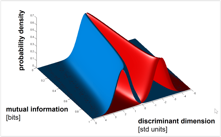
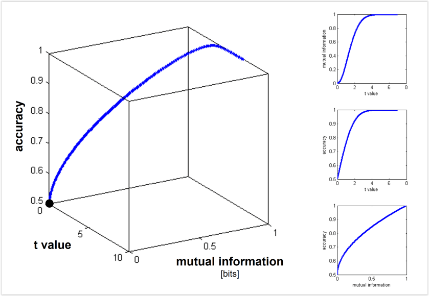
    Euclidean and Mahalanobis distance characterize the geometry (before or after whitening the noise, respectively). By contrast, saturating functions of these distances such as decoding accuracy or mutual information (for decoding stimulus pairs) do not optimally reflect the geometry. See Figs. 3, 4 below for the monotonic relationships among distance (measured along the Fisher linear discriminant), decoding accuracy, and mutual information between stimulus and response.
  • Should we use independent data to remove the positive bias of the dissimilarity estimate?
    Independent data (as in crossvalidation) can be used to remove the positive bias not only of the training-set accuracy of a decoder, but also of an estimate of a distance on the basis of noisy data (Kriegeskorte et al. 2007, Nili et al. 2014, Walther et al. 2016).

Linear decodability is widely used as a measure of representational distinctness, because decoding results are more relevant to neural computation when the decoder is biologically plausible for a single neuron. The advantages of linear decoding (interpretability, bias removal by crossvalidation) can be combined with the advantages of distances (non-quantization, non-saturation, characterization of representational geometry) and this is standardly done in representational similarity analysis by using the linear discriminant t (LD-t) value (Kriegeskorte et al. 2007, Nili et al. 2014) or the crossnobis estimator (Walther et al. 2016, Diedrichsen et al. 2016, Kriegeskorte & Diedrichsen 2016, Diedrichsen & Kriegeskorte 2017, Carlin et al. 2017). These measures of representational dissimilarity combine the advantages of decoding accuracies and continuous dissimilarity measures:

  • Biological plausibility: Like linear decoders, they reflect what can plausibly be directly read out.
  • Bias removal: As in linear decoding analyses, crossvalidation (1) removes the positive bias (which similarly affects training-set accuracies and distance functions applied to noisy data) and (2) provides robust frequentist tests of discriminability. For example, the crossnobis estimator provides an unbiased estimate of the Mahalanobis distance (Walther et al. 2016) with an interpretable 0 point.
  • Non-quantization: Unlike decoding accuracies, crossnobis and LD-t estimates are continuous estimates, uncompromised by quantization. Decoding accuracies, in contrast, are quantized by thresholding (based on often small counts of correct and incorrect predictions), which can reduce statistical efficiency (Walther et al. 2016).
  • Non-saturation: Unlike decoding accuracies, crossnobis and LD-t estimates do not saturate. Decoding accuracies suffer from a ceiling effect when two patterns that are already well-discriminable are moved further apart. Crossnobis and LD-t estimates proportionally reflect the true distances in the representational space.


gaussian separation -- mutual information
Figure 3: Gaussian separation for different values of the mutual information (in bits) between stimulus (binary: red, blue) and response. See slides for the First Cambridge Representational Similarity Analysis Workshop (http://www.mrc-cbu.cam.ac.uk/rsa2015/rsa2015media/).


t -- accuracy -- mutual information
Figure 4: Monotonic relationships among classifier accuracy, linear-discriminant t value (Nili et al. 2014), and bits of information (Kriegeskorte et al. 2007). See slides for the First Cambridge Representational Similarity Analysis Workshop (http://www.mrc-cbu.cam.ac.uk/rsa2015/rsa2015media/).


Strengths

  • The paper considers a wide range of dissimilarity measures (though these are not fully defined or explained).
  • The paper uses two fMRI data sets to compare many dissimilarity measures across many locations in the brain.

Weaknesses

  • The premise of the paper that optimal decoders are the gold standard does not make sense.
  • Even if decoding accuracy (e.g. linear) were taken as the standard to aspire to, why not use it directly, instead of a stand-in dissimilarity measure?
  • The paper lags behind the state of the literature, where researchers routinely use dissimilarity measures that are either based on decoding or that combine the advantages of decoding accuracies and continuous distances.

Major points

  • The premise that the optimal decoder should be the gold standard by which to choose a similarity measure does not make sense, because the optimal decoder reveals only the encoded information, but nothing about its format and what information is directly accessible to readout neurons.
  • If linear decoding accuracy (or the accuracy of some other simple decoder) is to be considered the gold standard measure of representational dissimilarity, then why not use the gold standard itself instead of a different dissimilarity measure?
  • In fact, representational similarity analyses using decoder accuracies and linear discriminability measures (LD-t, crossnobis) are widely used in the literature (Kriegeskorte et al. 2007, Nili et al. 2014, Cichy et al. 2014, Carlin et al. 2017 to name just a few).
  • One motivation for using the Pearson correlation distance to measure representational dissimilarity is to reduce the degree to which regional-mean activation differences affect the analyses. Researchers generally understand that Pearson correlation is not ideal from a decoding perspective, but prefer to choose a measure more complementary to regional-mean activation analyses. This motivation is inconsistent with the premise that decoder confusability should be the gold standard.
  • A better argument against using the Pearson correlation distance is that it has the undesirable property that it renders indistinguishable the case when two stimuli elicit very distinct response patterns and the case when neither stimulus drives the region strongly (and the pattern estimates are therefore noise and uncorrelated).

Is a cow-mug a cow to the ventral stream, and a mug to a deep neural network?

[I7R7]

An elegant new study by Bracci, Kalfas & Op de Beeck (pp2018) suggests that the prominent division between animate and inanimate things in the human ventral stream’s representational space is based on a superficial analysis of visual appearance, rather than on a deeper analysis of whether the thing before us is a living thing or a lifeless object.

Bracci et al. assembled a beautiful set of stimuli divided into 9 equivalent triads (Figure 1). Each triad consists of an animal, a manmade object, and a kind of hybrid of the two: an artefact of the same category and function as the object, designed to resemble the animal in the triad.

Screen Shot 08-16-18 at 05.52 PM 001
Figure 1: The entire set of 9 triads = 27 stimuli. Detail from Figure 1 of the paper.


Bracci et al. measured response patterns to each of the 27 stimuli (stimulus duration: 1.5 s) using functional magnetic resonance imaging (fMRI) with blood-oxygen-level-dependent (BOLD) contrast and voxels of 3-mm width in each dimension. Sixteen subjects viewed the images in the scanner while performing each of two tasks: categorizing the images as depicting something that looks like an animal or not (task 1) and categorizing the images as depicting a real living animal or a lifeless artefact (task 2).

The authors performed representational similarity analysis, computing representational dissimilarity matrices (RDMs) using the correlation distance (1 – Pearson correlation between spatial response patterns). They averaged representational dissimilarities of the same kind (e.g. between the animal and the corresponding hybrid) across the 9 triads. To compare different kinds of representational distance, they used ANOVAs and t tests to perform inference (treating the subject variable as a random effect). They also studied the representations of the stimuli in the last fully connected layers of two deep neural networks (DNNs; VGG-19, GoogLeNet) trained to classify objects, and in human similarity judgments. For the DNNs and human judgements, they used stimulus bootstrapping (treating the stimulus variable as a random effect) to perform inference.

Results of a series of well-motivated analyses are summarized in Figure 2 below (not in the paper). The most striking finding is that while human judgments and DNN last-layer representations are dominated by the living/nonliving distinction, human ventral temporal cortex (VTC) appears to care more about appearance: the hybrid animal-lookalike objects, despite being lifeless artefacts, fall closer to the animals than to the objects. In addition, the authors find:

  • Clusters of animals, hybrids, and objects: In VTC, animals, hybrids, and objects form significantly distinct clusters (average within-cluster dissimilarity < average between-cluster dissimilarity for all three pairs of categories). In DNNs and behavioral judgments, by contrast, the hybrids and the objects do not form significantly distinct clusters (but animals form a separate cluster from hybrids and from objects).
  • Matching of animals to corresponding hybrids: In VTC, the distance between a hybrid animal-lookalike and the corresponding animal is significantly smaller than that between a hydrid animal-lookalike and a non-matching animal. This indicates that VTC discriminates the animals and animal-lookalikes and (at least to some extent) matches the lookalikes to the correct animals. This effect was also present in the similarity judgments and DNNs. However, the latter two similarly matched the hybrids up with their corresponding objects, which was not a significant effect in VTC.


Screen Shot 08-16-18 at 05.52 PM
Figure 2: A qualitative visual summary of the results. Connection lines indicate different kinds of representational dissimilarity, illustrated for two triads although estimates and tests are based on averages across all 9 triads. Gray underlays indicate clusters (average within-cluster dissimilarity < average between-cluster dissimilarity, significant). Arcs indicate significantly different representational dissimilarities. It would be great if the authors added a figure like this in the revision of the paper. However, unlike the mock-up above, it should be a quantitatively accurate multidimensional scaling (MDS, metric stress) arrangement, ideally based on unbiased crossvalidated representational dissimilarity estimates.


The effect of the categorization task on the VTC representation was subtle or absent, consistent with other recent studies (cf. Nastase et al. 2017, open review). The representation appears to be mostly stimulus driven.

The results of Bracci et al. are consistent with the idea that the ventral stream transforms images into a semantic representation by computing features that are grounded in visual appearance, but correlated with categories (Jozwik et al. 2015). VTC might be 5-10 nonlinear transformations removed from the image. While it may emphasize visual features that help with categorization, it might not be the stage where all the evidence is put together for our final assessment of what we’re looking at. VTC, thus, is fooled by these fun artefacts, and that might be what makes them so charming.

Although this interpretation is plausible enough and straightforward, I am left with some lingering thoughts to the contrary.

What if things were the other way round? Instead of DNNs judging correctly where VTC is fooled, what if VTC had a special ability that the DNNs lack: to see the analogy between the cow and the cow-mug, to map the mug onto the cow? The “visual appearance” interpretation is based on the deceptively obvious assumption that the cow-mug (for example) “looks like” a cow. One might, equally compellingly, argue that it looks like a mug: it’s glossy, it’s conical, it has a handle. VTC, then, does not fail to see the difference between the fake animal and the real animal (in fact these categories do cluster in VTC). Rather it succeeds at making the analogy, at mapping that handle onto the tail of a cow, which is perhaps an example of a cognitive feat beyond current AI.

Bracci et al.’s results are thought-provoking and the study looks set to inspire computational and empirical follow-up research that links vision to cognition and brain representations to deep neural network models.


Strengths

  • addresses an important question
  • elegant design with beautiful stimulus set
  • well-motivated and comprehensive analyses
  • interesting and thought-provoking results
  • two categorization tasks, promoting either the living/nonliving or the animal-appearance/non-animal appearance division
  • behavioral similarity judgment data
  • information-based searchlight mapping, providing a broader view of the effects
  • new data set to be shared with the community


Weaknesses

  • representational geometry analyses, though reasonable, are suboptimal
  • no detailed analyses of DNN representations (only the last fully connected layers shown, which are not expected to best model the ventral stream) or the degree to which they can explain the VTC representation
  • only three ROIs (V1, posterior VTC, anterior VTC)
  • correlation distance used to measure representational distances (making it difficult to assess which individual representational distances are significantly different from zero, which appears important here)


Suggestions for improvement

The analyses are effective and support most of the claims made. However, to push this study from good to excellent, I suggest the following improvements.


Major points

Improved representational-geometry analysis

The key representational dissimilarities needed to address the questions of this study are labeled a-g in Figure 2. It would be great to see these seven quantities estimated, tested for deviation from 0, and all 7 choose 2 = 21 pairwise comparisons tested. This would address which distinctions are significant and enable addressing all the questions with a consistent approach, rather than combining many qualitatively different statistics (including clustering index, identity index, and model RDM correlation).

With the correlation distance, this would require a split-data RDM approach, consistent with the present approach, but using the repeated response measurements to the same stimulus to estimate and remove the positive bias of the correlation-distance estimates. However, a better approach would be to use a crossvalidated distance estimator (more details below).


Multidimensional scaling (MDS) to visualize representational geometries

This study has 27 unique stimuli, a number well suited for visualization of the representational geometries by MDS. To appreciate the differences between the triads (each of which has unique features), it would be great to see an MDS of all 27 objects and perhaps also MDS arrangements of subsets, e.g. each triad or pairs of triads (so as to reduce distortions due to dimensionality reduction).

Most importantly, the key representational dissimilarities a-g can be visualized in a single MDS as shown in Figure 2 above, using two triads to illustrate the triad-averaged representational geometry (showing average within- and between-triad distances among the three types of object). The MDS could use 2 or 3 dimensions, depending on which variant better visually conveys the actual dissimilarity estimates.


Crossvalidated distance estimators

The correlation distance is not an ideal dissimilarity measure because a large correlation distance does not indicate that two stimuli are distinctly represented. If a region does not respond to either stimulus, for example, the correlation of the two patterns (due to noise) will be close to 0 and the correlation distance will be close to 1, a high value that can be mistaken as indicating a decodable stimulus pair.

Crossvalidated distances such as the linear-discriminant t value (LD-t; Kriegeskorte et al. 2007, Nili et al. 2014) or the crossnobis distance (also known as the linear discriminant contrast, LDC; Walther et al. 2016) would be preferable. Like decoding accuracy, they use crossvalidation to remove bias (due to overfitting) and indicate that the two stimuli are distinctly encoded. Unlike decoding accuracy, they are continuous and nonsaturating, which makes them more sensitive and a better way to characterize representational geometries.

Since the LD-t and the crossnobis distance estimators are symmetrically distributed about 0 under the null hypothesis (H0: response patterns drawn from the same distribution), it would be straightforward to test these distances (and averages over sets of them) for deviation from 0, treating subjects and/or stimuli as random effects, and using t tests, ANOVAs, or nonparametric alternatives. Comparing different dissimilarities or set-average dissimilarities is similarly straightforward.


Linear crossdecoding with generalization across triads

An additional analysis that would give complementary information is linear decoding of categorical divisions with generalization across stimuli. A good approach would be leave-one-triad-out linear classification of:

  • living versus nonliving
  • things that look like animals versus other things
  • animal-lookalikes versus other things
  • animals versus animal-lookalikes
  • animals versus objects
  • animal-lookalikes versus objects

This might work for devisions that do not show clustering (within dissimilarity < between dissimilarity), which would indicate linear separability in the absence of compact clusters.

For the living/nonliving destinction, for example, the linear discriminant would select responses that are not confounded by animal-like appearance (as most VTC responses seem to be), responses that distinguish living things from animal-lookalike objects. This analysis would provide a good test of the existence of such responses in VTC.


More layers of the two DNNs

To assess the hypothesis that VTC computes features that are more visual than semantic with DNNs, it would be useful to include an analysis of all the layers of each of the two DNNs, and to test whether weighted combinations of layers can explain the VTC representational geometry (cf. Khaligh-Razavi & Kriegeskorte 2014).


More ROIs

How do these effects look in V2, V4, LOC, FFA, EBA, and PPA?


Minor points

The use of the term “bias” in the abstract and main text is nonstandard and didn’t make sense to me. Bias only makes sense when we have some definition of what the absence of bias would mean. Similarly the use of “veridical” in the abstract doesn’t make sense. There is no norm against which to judge veridicality.


The polar plots are entirely unmotivated. There is no cyclic structure or even meaningful order to the the 9 triads.


“DNNs are very good, and even better than than human visual cortex, at identifying a cow-mug as being a mug — not a cow.” This is not a defensible claim for several reasons, each of which by itself suffices to invalidate this.

  • fMRI does not reveal all the information in cortex.
  • VTC is not all of visual cortex.
  • VTC does cluster animals separately from animal-lookalikes and from objects.
  • Linear readout of animacy (cross-validated across triads) might further reveal that the distinction is present (even if it is not dominant in the representational geometry.


Grammar, typos

“how an object looks like” -> ‘how an object looks” or “what an object looks like”

“as oppose to” -> “as opposed to”

“where observed” -> “were observed”


Discrete-event-sequence model reveals the multi-time-scale brain representation of experience and recall

[I8R7]

Baldassano, Chen, Zadbood, Pillow, Hasson & Norman (pp2016) investigated brain representations of event sequences with fMRI. The paper argues in favour of an intriguing and comprehensive account of the representation of event sequences in the brain as we experience them, their storage in episodic memory, and their later recall.

The overall story is quite amazing and goes like this: Event sequences are represented at multiple time scales across brain regions during experience. The brain somehow parses the continuous stream of experience into discrete pieces, called events. This temporal segmentation occurs at multiple temporal scales, corresponding perhaps to a tree of higher-level (longer) events and subevents. Whether the lower-level events precisely subdivide higher-level events (rendering the multiscale structure a tree) is an open question, but at least different regions represent event structure at different scales. Each brain region has its particular time scale and represents an event as a spatial pattern of activity. The encoding in episodic memory does not occur continuously, but rather in bursts following the event transitions at one of the longer time scales. During recall from memory, the event representations are reinstated, initially in the higher-level regions, from which the more detailed temporal structure may come to be associated in the lower-level regions. Event representations can arise from perceptual experience (a movie here), recall (telling the story), or from listening to a narration. If the event sequence of a narration is familiar, memory recall can help reinstate representations upcoming in the narration in advance.

There’s previous evidence for event segmentation (Zacks et al. 2007) and multi-time-scale representation (from regional-mean activation to movies that are temporally scrambled at different temporal scales; Hasson et al. 2008; see also Hasson et al. 2015) and for increased hippocampal activity at event boundaries (Ben-Yakov et al. 2013). However, the present study investigates pattern representations and introduces a novel model for discovering the inherent sequence of event representations in regional multivariate fMRI pattern time courses.

The model assumes that a region represents each event k = 1..K as a static spatial pattern mk of activity that lasts for the duration of the event and is followed by a different static pattern mk+1 representing the next event. This idea is formalised in a Hidden Markov Model with K hidden states arranged in sequence with transitions (to the next time point) leading either to the same state (remain) or to the next state (switch). Each state k is associated with a regional activity pattern mk, which remains static for the duration of the state (the event). The number of events for a given region’s representation of, say, 50 minutes’ experience of a movie is chosen so as to maximise within-event minus between-event pattern correlation on a held-out subject.

It’s a highly inspired paper and a fun read. Many of the analyses are compelling. The authors argue for such a comprehensive set of claims that it’s a tall order for any single paper to fully substantiate all of them. My feeling is that the authors are definitely onto something. However, as usual there may be alternative explanations for some of the results and I am left with many questions.


Strengths

  • The paper is very ambitious, both in terms brain theory and in terms of analysis methodology.
  • The Hidden Markov Model of event sequence representation is well motivated, original, and exciting. I think this has great potential for future studies.
  • The overall account of multi-time-scale event representation, episodic memory encoding, and recall is plausible and fascinating.


Weaknesses

  • Incomplete description and validation of the new method: The Hidden Markov Model is great and quite well described. However, the paper covers a lot of ground, both in terms of the different data sets, the range of phenomena tackled (experience, memory, recall, multimodal representation, memory-based prediction), the brain regions analysed (many regions across the entire brain), and the methodology (novel complex method). This is impressive, but it also means that there is not much space to fully explain everything. As a result there are several important aspects of the analysis that I am not confident I fully understood. It would be good to describe the new method in a separate paper where there is enough space to validate and discuss it in detail. In addition, the present paper needs a methods figure and a more step-by-step description to explain the pattern analyses.
  • The content and spatial grain of the event representations is unclear. The analyses focus on the sequence of events and the degree to which the measured pattern is more similar within than between inferred event boundaries. Although this is a good idea, I would have more confidence in the claims if the content of the representations was explicitly investigated (e.g. representational patterns that recur during the movie experience could represent recurring elements of the scenes).
  • Not all claims are fully justified. The paper claims that events are represented by static patterns, but this is a model assumption, not something demonstrated with the data. It’s also claimed that event boundaries trigger storage in long-term memory, but hippocampal activity appears to rise before event boundaries (with the hemodynamic peak slightly after the boundaries). The paper could even more clearly explain exactly what previous studies showed, what was assumed in the model (e.g. static spatial activity patterns representing the current event) and what was discovered from the data (event sequence in each region).


Particular points the authors may wish to address in revision

 (1) Do the analyses reflect fine-grained pattern representations?

The description of exactly how evidence is related between subjects is not entirely clear. However, several statements suggest that the analysis assumes that representational patterns are aligned across subjects, such that they can be directly compared and averaged across subjects. The MNI-based intersubject correspondency is going to be very imprecise. I would expect that the assumption of intersubject spatial correspondence lowers the de facto resolution from 3 mm to about a centimetre. The searchlight was a very big (7 voxels = 2.1cm)3 cube, so perhaps still contained some coarse-scale pattern information.

However, even if there is evidence for some degree of intersubject spatial correspondence (as the authors say results in Chen et al. 2016 suggest), I think it would be preferable to perform the analyses in a way that is sensitive also to fine-grained pattern information that does not align across subjects in MNI space. To this end patterns could be appended, instead of averaged, across subjects along the spatial (i.e. voxel) dimension, or higher-level statistics, such as time-by-time pattern dissimilarities, could averaged across subjects.

If the analyses really rely on MNI intersubject correspondency, then the term “fine-grained” seems inappropriate. In either case, the question of the grain of the representational patterns should be explicitly discussed.


(2) What is the content of the event representations?

The Hidden Markov Model is great for capturing the boundaries between events. However, it does not capture the meaning and relationships between the event representations. It would be great to see the full time-by-time representational dissimilarity matrices (RDMs; or pattern similarity matrices) for multiple regions (and for single subjects and averaged across subjects). It would also be useful to average the dissimilarities within each pair of events to obtain event-by-event RDMs. These should reveal, when events recur in the movie, and the degree of similarity of different events in each brain region. If each event were unique in the movie experience, these RDMs would have a diagonal structure. Analysing the content of the event representations in some way seems essential to the interpretation that the patterns represent events.


(3) Why do the time-by-time pattern similarity matrices look so low-dimensional?

The pattern correlations shown in Figure 2 for precuneus and V1 are very high in absolute value and seem to span the entire range from -1 to 1. (Are the patterns averaged across all subjects?) It looks like two events either have highly correlated or highly anticorrelated patterns. This would suggest that there are only two event representations and each event falls into one of two categories. Perhaps there are intermediate values, but the structure of these matrices looks low-dimensional (essentially 1 dimensional) to me. The strong negative correlations might be produced by the way the data are processed, which could be more clearly described. For example, if the ensemble of patterns were centered in the response space by subtracting the mean pattern from each pattern, then strong negative correlations would arise.

I am wondering to what extent these matrices might reflect coarse-scale overall activation fluctuations rather than detailed representations of individual events. The correlation distance removes the mean from each pattern, but usually different voxels respond with different gains, so activation scales rather than translates the pattern up. When patterns are centered in response space, 1-dimensional overall activation dynamics can lead to the appearance of correlated and anticorrelated pattern states (along with intermediate correlations) as seen here.

This concern relates also to points (1) and (2) above and could be addressed by analysing fine-grained within-subject patterns and the content of the event representations.

screenshot1350

Detail from Figure 2: Time-by-time regional spatial-pattern correlation matrices.
Precuneus (top) and V1 (bottom).


(4) Do brain regions really represent a discrete sequence of events by a discrete sequence of patterns?

The paper currently claims to show that brain regions represent events as static patterns, with sudden switches at the event boundaries. However, this is not something that is demonstrated from the data, rather it is the assumption built into the Hidden Markov Model.

I very much like the Hidden Markov Model, because it provides a data-driven way to discover the event boundaries. The model assumption of static patterns and sudden switches are fine for this purpose because they may provide an approximation to what is really going on. Sudden switches are plausible, since transitions between events are sudden cognitive phenomena. However, it seems unlikely that patterns are static within events. This claim should be removed or substantiated by an inferential comparison of the static-pattern sequence model with an alternative model that allows for dynamic patterns within each event.


(5) Why use the contrast of within- and between-event pattern correlation in held-out subjects as the criterion for evaluating the performance of the Hidden Markov Model?

If patterns are assumed to be aligned between subjects, the Hidden Markov Model could be used to directly predict the pattern time course in a held-out subject. (Predicting the average of the training subjects’ pattern time courses would provide a noise ceiling.) The within- minus between-event pattern correlation has the advantage that it doesn’t require the assumption of intersubject pattern alignment, but this advantage appears not to be exploited here. The within- minus between-event pattern correlation seems problematic here because patterns acquired closer in time tend to be more similar (Henriksson et al. 2015). First, the average within-event correlation should always tend to be larger than the average between-event correlation (unless the average between-event correlation were estimated from the same distribution of temporal lags). Such a positive bias would be no problem for comparing between different segmentations. However, if temporally close patterns are more similar, then even in the absence of any event structure, we expect that a certain number of events best captures the similarity among temporally closeby patterns. The inference of the best number of events would then be biased toward the number of events, which best captures the continuous autocorrelation.


(6) More details on the recall reactivation

Fig. 5a is great. However, this is a complex analysis and it would be good to see this in all subjects and to also see the movie-to-recall pattern similarity matrix, with the human annotations-based and Hidden Markov Model-based time-warp trajectories superimposed. This would enable us to better understand the data and how the Hidden Markov Model arrives at the assignment of corresponding events.

In addition, it would be good to show statistically, that the Hidden Markov Model predicts the content correspondence between movie and recall representations consistently with the human annotations.


(7) fMRI is a hemodynamic measure, not “neural data”.

“Using a data-driven event segmentation model that can identify temporal structure directly from neural measurements”; “Our results are the first to demonstrate a number of key predictions of event segmentation theory (Zacks et al., 2007) directly from neural data”

There are a couple of other places, where “neural data” is used. Better terms include “fMRI data” and “brain activity patterns”.


(8) Is the structure of the multi-time-scale event segmentation a tree?

Do all regions that represent the same time-scale have the same event boundaries? Or do they provide alternative temporal segmentations? If it is the former, do short-time-scale regions strictly subdivide the segmentation of longer-time-scale regions, thus making the event structure a tree? Fig. 1 appears to be designed so as not to imply this claim. Data, of course, is noisy, so we don’t expect a perfect tree to emerge in the analysis, even if our brains did segment experience into a perfect tree. It would be good to perform an explicit statistical comparison between the temporal-tree event segmentation hypothesis and the more general multi-time-scale event segmentation hypothesis.


(9) Isn’t it a foregone conclusion that longer-time-scale regions’ temporal boundaries will match better to human annotated boundaries?

“We then measured, for each brain searchlight, what fraction of its neurally-defined boundaries were close to (within three time points of) a human-labeled event boundary.”

For a region with twice as many boundaries as another region, this fraction is halved even if both regions match all human labeled events. This analysis therefore appears strongly confounded by the number of events a regions represents.

The confound could be removed by having humans segment the movie at multiple scales (or having them segment at a short time scale and assign saliency ratings to the boundaries). The number of events could then be matched before comparing segmentations between human observers and brain regions.

Conversely, and without requiring more human annotations, the HMM could be constrained to the number of events labelled by humans for each searchlight location. This would ensure that the fraction of matches to human observers’ boundaries can be compared between regions.


(10) Hippocampus response does not appear to be “triggered” by the end of the event, but starts much earlier.

The hemodynamic peak is about 2-3 s after the event boundary, so we should expect the neural activity to begin well before the event boundary.


(11) Is the time scale a region represents reflected in the temporal power spectrum of spontaneous fluctuations?

The studies presenting such evidence are cited, but it would be good to look at the temporal power spectrum also for the present data and relate these two perspectives. I don’t think the case for event representation by static patterns is quite compelling (yet). Looking at the data also from this perspective may help us get a fuller picture.


(12) The title and some of the terminology is ambiguous

The title “Discovering event structure in continuous narrative perception and memory” is, perhaps intentionally, ambiguous. It is unclear who or what “discovers” the event structure. On the one hand, the brain that discovers event structure in the stream of experience. On the other hand, the Hidden Markov Model discovers good segmentations of regional pattern time courses. Although both interpretations work in retrospect, I would prefer a title that makes a point that’s clear from the beginning.

On a related note, the phrase “data-driven event segmentation model” suggests that the model performs the task of segmenting the sensory stream into events. This was initially confusing to me. In fact, what is used here is a brain-data-driven pattern time course segmentation model.


(13) Selection bias?

I was wondering about the possibility of selection bias (showing the data selected by brain mapping, which is biased by the selection process) for some of the figures, including Figs. 2, 4, and 7. It’s hard to resist illustrating the effects by showing selected data, but it can be misleading. Are the analyses for single searchlights? Could they be crossvalidated?


(14) Cubic searchlight

A spherical or surface-based searchlight would the better than a (2.1 cm)3 cube.


– Nikolaus Kriegeskorte


Acknowledgement

I thank Aya Ben-Yakov for discussing this paper with me.


Brain representations of animal videos are surprisingly stable across tasks and only subtly modulated by attention

[R7I7]

Nastase et al. (pp2016) presented video clips (duration: 2 s) to 12 human subjects during fMRI. In a given run, a subject performed one of two tasks: detecting repetitions of either the animal’s behaviour (eating, fighting, running, swimming) or the category of animal (primate, ungulate, bird, reptile, insect). They performed region-of-interest and searchlight-based pattern analyses. Results suggest that:

  • The animal behaviours are associated with clearly distinct patterns of activity in many regions, whereas different animal taxa are less discriminable overall. Within-animal-category representational dissimilarities (correlation distances) are similarly large as between-animal-category representational dissimilarities, indicating little clustering by these (very high-level) animal categories. However, animal-category decoding is above chance in a number of visual regions and generalises across behaviours, indicating some degree of linear separability. For the behaviours, there is strong evidence for both category clustering and linear separability (decodability generalising across animal taxa).
  • Representations are remarkably stable across attentional tasks, but subtly modulated by attention in higher regions. There is some evidence for subtle attentional modulations, which (as expected) appear to enhance task-relevant sensory signals.

Overall, this is a beautifully designed experiment and the analyses are comprehensive and sophisticated. The interpretation in the paper focusses on the portion of the results that confirms the widely accepted idea that task-relevant signals are enhanced by attention. However, the stability of the representations across attentional tasks is substantial and deserves deeper analyses and interpretation.


screenshot1195

Spearman correlations between regional RDMs and behaviour-category RDM (top) and a animal-category RDM (bottom). These correlations measure category clustering in the representation. Note (1) that clustering is strong for behaviours but weak for animal taxa, and (2) that modulations of category clustering are subtly, but significant in several regions, notably in the left postcentral sulcus (PCS) and ventral temporal (VT) cortex.


Strengths

  • The experiment is well motivated and well designed. The movie stimuli are naturalistic and likely to elicit vivid impressions and strong responses. The two attentional tasks are well chosen as both are quite natural. There are 80 stimuli in total: 5 taxa * 4 behaviours * 2 particular clips * 2 horizontally flipped versions. It’s impossible to control confounds perfectly with natural video clips, but this seems to strike quite a good balance between naturalism and richness of sampling and experimental control.
  • The analyses are well motivated, sophisticated, well designed, systematic and comprehensive. Analyses include both a priori ROIs (providing greater power through fewer tests) and continuous whole-brain maps of searchlight information (giving rich information about the distribution of information across the brain). Surface-based searchlight hyperalignment based on a separate functional dataset ensures good coarse-scale alignment between subjects (although detailed voxel pattern alignment is not required for RSA). The cortical parcellation based on RDM clustering is also an interesting feature. The combination of threshold-free cluster enhancement and searchlight RSA is novel, as far as I know, and a good idea.


Weaknesses

  • The current interpretation mainly confirms prevailing bias. The paper follows the widespread practice in cognitive neuroscience of looking to confirm expected effects. The abstract tells us what we already want to believe: that the representations are not purely stimulus driven, but modulated by attention and in a way that enhances the task-relevant distinctions. There is evidence for this in previous studies, for simple controlled stimuli, and in the present study, for more naturalistic stimuli. However, the stimulus, and not the task, explains the bulk of the variance. It would be good to engage the interesting wrinkles and novel information that this experiment could contribute, and to describe the overall stability and subtle task-flexibility in a balanced way.
  • Behavioural effects confounded with species: Subjects saw a chimpanzee eating a fruit, but they never saw that chimpanzee, or in fact any chimpanzee fighting. The videos showed different animal species in the primate category. Effects of the animal’s behaviour, thus, are confounded with species effects. There is no pure comparison between behaviours within the same species and/or individual animal. It’s impossible to control for everything, but the interpretation requires consideration of this confound, which might help explain the pronounced distinctness of clips showing different behaviours.
  • Asymmetry of specificity between behaviours and taxa: The behaviours were specific actions, which correspond to linguistically frequent action concepts (eating, fighting, running, swimming). However, the animal categories were very general (primate, ungulate, bird, reptile, insect), and within each animal category, there were different species (corresponding roughly to linguistically frequent basic-level noun concepts). The fact that the behavioural but not the animal categories corresponded to linguistically frequent concepts may help explain the lack of animal-category clustering.
  • Representational distances were measured with the correlation distance, creating ambiguity. Correlation distances are ambiguous. If they increase (e.g. for one task as compared to another) this could mean (1) the patterns are more discriminable (the desired interpretation), (2) the overall regional response (signal) was weaker, or (3) the noise was greater; or any combination of these. To avoid this ambiguity, a crossvalidated pattern dissimilarity estimator could be used, such as the LD-t (Kriegeskorte et al. 2007; Nili et al. 2014) or the crossnobis estimator (Walther et al. 2015; Diedrichsen et al. pp2016; Kriegeskorte & Diedrichsen 2016). These estimators are also more sensitive (Walther et al. 2015) because, like the Fisher linear discriminant, they benefit from optimal weighting of the evidence distributed across voxels and from noise cancellation between voxels. Like decoding accuracies, these estimators are crossvalidated, and therefore unbiased (in particular, the expected value of the distance estimate is zero under the null hypothesis that the patterns for two conditions are drawn from the same distribution). Unlike decoding accuracies, these distance estimators are continuous and nonsaturating, providing a more sensitive and undistorted characterisation of the representational geometry.
  • Some statistical analysis details are missing or unclear. The analyses are complicated and not everything is fully and clearly described. In several places the paper states that permutation tests were used. This is often a good choice, but not a sufficient description of the procedure. What was the null hypothesis? What entities are exchangeable under that null hypothesis? What was permuted? What exactly was the test statistic? The contrasts and inferential thresholds could be more clearly indicated in the figures. I did not understand in detail how searchlight RSA and threshold-free cluster enhancement were combined and how map-level inference was implemented. A more detailed description should be added.
  • Spearman RDM correlation is not optimally interpretable. Spearman RDM correlation is used to compare the regional RDMs with categorical RDMs for either behavioural categories or animal taxa. Spearman correlation is not a good choice for model comparisons involving categorical models, because of the way it deals with ties, of which there are many in categorical model RDMs (Nili et al. 2014). This may not be an issue for comparing Spearman RDM correlations for a single category-model RDM between the two tasks. However, it is still a source of confusion. Since these model RDMs are binary, I suspect that Spearman and Pearson correlation are equivalent here. However, for either type of correlation coefficient, the resulting effect size depends on the proportion of large distances in the model matrix (30 of 190 for the taxonomy and 40 of 190 for the behavioural model). Although I think it is equivalent for the key statistical inferences here, analyses would be easier to understand and effect sizes more interpretable if differences between averages of dissimilarities were used.


Suggestions

In general, the paper is already at a high level, but the authors may consider making improvements addressing some of the weaknesses listed above in a revision. I have a few additional suggestions.

  • Open data: This is a very rich data set that cannot be fully analysed in a single paper. The positive impact on the field would be greatest if the data were made publicly available.
  • Structure and clarify the results section: The writing is good in general. However, the results section is a long list of complex analyses whose full motivation remains unclear in some places. Important details for basic interpretation of the results should be given before stating the results. It would be good to structure the results section according to clear claims. In each subsection, briefly state the hypothesis, how the analysis follows from the hypothesis, and what assumptions it depends on, before describing the results.
  • Compare regional RDMs between tasks without models: It would be useful to assess whether representational geometries change across tasks without relying on categorical model RDMs. To this end the regional RDMs (20×20 stimuli) could be compared between tasks. A good index to be computed for each subject would be the between-task RDM correlation minus the within-task RDM correlation (both across runs and matched to equalise the between run temporal separation). Inference could use across subject nonparametric methods (subject as random effect). This analysis would reveal the degree of stability of the representational geometry across tasks.
  • Linear decoding generalising across tasks: It would be good to train linear decoders for behaviours and taxa in one task and test for generalisation to the other task (and simultaneously across the other factor).
  • Independent definition of ROIs: Might the functionally driven parcellation of the cortex and ROI selection based on intersubject searchlight RDM reliability not bias the ROI analyses? It seems safer to use independently defined ROIs.
  • Task decoding: It would be interesting to see a searchlight maps of task decodability. Training and test sets should always consist of different runs. One could assess generalisation to new runs and ideally also generalisation across behaviours and taxa (leaving out one animal category or one behavioural category from the training set).
  • Further investigate the more prominent distinctions among behaviours than among taxa: Is this explained by a visual similarity confound? Cross-decoding of behaviour between taxa sheds some light on this. However, it would be good also to analyse the videos with motion-energy models and look at the representational geometries in such models.


Additional specific comments and questions

Enhancement and collapse have not been independently measured. The abstract states: “Attending to animal taxonomy while viewing the same stimuli increased the discriminability of distributed animal category representations in ventral temporal cortex and collapsed behavioural information.” Similarly, on page 12, it says: “… accentuating task-relevant distinctions and reducing unattended distinctions.”
This description is intuitive, but it incorrectly suggests that the enhancement and collapse have been independently measured. This is not the case: It would require a third, e.g. passive-viewing condition. Results are equally consistent with the interpretation that attention just enhances the task-relevant distinctions (without collapsing anything). Conversely, the reverse might also be consistent with the results shown: that attention just collapses the task-irrelevant distinctions (without enhancing anything).

You explain in the results that this motivates the use of the term categoricity, but then don’t use that term consistently. Instead you describe it as separate effects, e.g. in the abstract.

The term categoricity may be problematic for other reasons. A better description might be “relative enhancement of task-relevant representational distinctions”. Results would be more interpretable if crossvalidated distances were used, because this would enable assessment of changes in discriminability. By contrast, larger correlation distance can also result from reduced responses or nosier data.


Map-inferential thresholds are not discernable: In Fig. 2, all locations with positively model-correlated RDMs are marked in red. The locations exceeding the map-inferential threshold are not visible because the colour scale uses red for below- and above-threshold values. The legend (not just the methods section) should also clarify whether multiple testing was corrected for and if so how. The Fig. 2 title “Effect of attention on local representation of behaviour and taxonomy” is not really appropriate, since the inferential results on that effect are in Fig. S3. Fig. S3 might deserve to be in the main paper, given that the title claim is about task effects.


Videos on YouTube: To interpret these results, one really has to watch the 20 movies. How about putting them on YouTube?


Previous work: The work of Peelen and Kastner and of Sigala and Logothetis on attentional dependence of visual representations should be cited and discussed.


Colour scale: The jet colour scale is not optimal in general and particularly confusing for the model RDMs. The category model RDMs for behaviour and taxa seem to contain zeroes along the diagonal, ones for within-category comparisons and twos for between-category comparisons. Is the diagonal excluded from model? In that case the matrix is binary, but contains ones and twos instead of zeroes and ones. While this doesn’t matter for the correlations, it is a source of confusion for readers.


Show RDMs: To make results easier to understand, why not show RDMs? Could average certain sets of values for clarity.


Statistical details

“When considering all surviving searchlights for both attention tasks, the mean regression coefficient for the behavioural category target RDM increased significantly from 0.100 to 0.129 (p = .007, permutation test).”
Unclear: What procedure do these searchlights “survive”? Also: what is the null hypothesis? What is permuted? Are these subject RFX tests?

The linear mixed effects model of Spearman RDM correlations suggests differences between regions. However, given the different noise levels between regions, I’m not sure these results are conclusive (cf. Diedrichsen et al. 2011).

“To visualize attentional changes in representational geometry, we first computed 40 × 40 neural RDMs based on the 20 conditions for both attention tasks and averaged these across participants.”
Why is the 40×40 RDM (including, I understand, both tasks) ever considered? The between-task pattern comparisons are hard to interpret because they were measured in different runs (Henriksson et al. 2015; Alink et al. pp2015).

“Permutation tests revealed that attending to animal behaviour increased correlations between the observed neural RDM and the behavioural category target RDM in vPC/PM (p = .026), left PCS (p = .005), IPS (p = .011), and VT (p = .020).”
What was the null? What was permuted? Do these survive multiple testing correction? How many regions were analysed?

Fig. 3: Bootstrapped 95% confidence intervals. What was bootstrapped? Conditions?

page 14: Mean of searchlight regression coefficients – why only select those searchlights that survive TFCE in both attention conditions?

page 15: Parcellation of ROIs based on the behaviour attention data only. Why?

SI text: Might eye movements constitute a confound? (Free viewing during video clips)

“more unconfounded” -> “less confounded”


Acknowledgement
Thanks to Marieke Mur for discussing this paper with me and sharing her comments, which are included above.

— Nikolaus Kriegeskorte