Tomoyasu Horikawa presents a method called “mind captioning” for decoding perceptual and cognitive content in the form of English text from human brain activity measured with functional MRI (brain-to-text: b2t). Brain-to-text decoding is an important concept because of the versatility and universality of language: It promises to enable us to read out all kinds of brain representations (not just those of linguistic content) and thus has broad potential for neuroscience and applications requiring brain-machine interfaces.
The author relied on human annotators to generate multiple verbal captions describing each of thousands of videos (video-to-text: v2t). He fed these text captions to a neural-network language model to obtain a compressed semantic feature vector characterizing the content of each video (text-to-features: t2f). He trained an L2-regularized linear decoder for each semantic feature to predict the features from human brain activity measured with functional MRI (fMRI) while subjects watched videos (brain-to-features: b2f). He then converted the features to text (features-to-text: f2t) using an iterative text synthesis procedure to invert the t2f mapping.
This iterative evolutionary text synthesis procedure is an important contribution. It proceeds from a seed (such as an uninformative token), iteratively replacing words so as to improve the correlation between the semantic feature vector predicted by the text-to-feature language model and the feature vector decoded from brain activity. The mutated captions considered are constructed by masking out particular words and then generating potential replacements using another language model (RoBERTa-large) that has been trained with masking of tokens to predict missing tokens. This masked language model provides probable completions and thus constrains the search to natural text descriptions, while the candidate descriptions best matching the decoded features are selected for further optimization.
The study also applies the decoder not only to brain activity measured while subjects view videos, but also to activity measured while subjects recall and imagine videos they previously viewed. Recall-based imagery can be decoded at levels far above chance, though much lower than perception, in high-level visual cortex. Careful encoding and decoding analyses demonstrate that information about the videos is widespread throughout the human cortex, including in the language network. However, excluding the language network for decoding did not substantially reduce decoding performance. This is a key result because the goal of brain-to-text decoding is not the decoding of verbal thoughts, but the use of text to capture the information in all kinds of brain representations, most of which are not verbal. Language is an excellent format for decoding because it can capture concrete as well as abstract information. Unlike a decoder that outputs images, a text decoder can leave out information that is unspecified in the representation being decoded.
A central claim of the study is that the results support the hypothesis that high-level visual cortex contains structured semantic representations that capture not only the sets of objects present in the scene but also their relationships (such as “man bites dog” as opposed to “dog bites man”). In addition, the author suggests that the text synthesis approach enables “faithful” decoding unbiased, or at least less biased, by prior knowledge than previous approaches (e.g. using a caption database).
Overall, this is excellent work, tackling a grand decoding challenge with many original and inspiring ideas which are expertly implemented. The analyses in the main paper and the supplementary analyses are careful and comprehensive. The examples of decoded text are impressive. However, the claim of “faithful” or “unbiased” decoding does not make sense to me. Arguably it is not even desirable to decode without prior information (i.e. without bias): To understand what the information in the brain “means”, we need to interpret it in light of what we know about the world. After all, the rest of the brain that is using the representation is also interpreting it in the context of what it knows about the world. The author should either rigorously justify these claims or leave them out.
The claims about structured semantic representation and representation of relationships may also need to be tempered a bit. I am unsure if the word shuffling analyses supporting this claim may be compromised by the fact that the resulting text is not within the distribution that the text-to-feature language model was trained on. Really addressing the structured relational semantics hypothesis would require out-of-distribution tests such as a video of a man biting a dog (an example the author introduces in the discussion), whose decoding might reveal to what extent the decoder relies on the brain representation and to what extent it infers the structure in the decoded text using its prior knowledge of the world. The paper could also be further improved by discussing the motivations for the choices made in designing the decoder and alternative choices and why they are promising or not promising.
Even if some of the claims need adjustment, this is an excellent and highly original contribution that will be of broad interest to neuroscientists and researchers in other fields.
Suggestions
Fully justify or weaken claims of “faithful” decoding unbiased by prior information.
Add a figure and table clarifying the different formats of information (video, visual features, captions, semantic features, brain activity) and all the transformations (v2t by humans, t2f by language models, b2f by linear decoder, f2t by iterative text synthesis).
Add a section to the discussion motivating the particular choices for these transformations. For example, why should brain activity and text be aligned at the level of the semantic features? Why not learn to map directly from brain activity to text? Why use an interactive inversion of the t2f model, rather than learning a direct f2t mapping? How well does the text-to-feature model preserve the information in the text? If presented with the feature vectors corresponding to a set of independent draws from the training distribution of captions (different captions, but IID), how well does the optimization method recover the description? How much of the information in the recovered verbal description is encoded in the semantic features and how much comes from the prior implicit to the text-to-feature encoder?
Add a section to the discussion addressing whether “faithful” or “unbiased” decoding is even well-defined as an ideal – whether or not it is achievable in practice.
Strengths
The paper addresses an inspiring and important challenge with scientific and applied dimensions.
Decoders are applied not only to data acquired during the viewing of videos, but also during memory-recall-driven mental imagery.
The iterative text synthesis decoding procedure is original and powerful.
The methods are original and state of the art.
The encoding and decoding analyses are comprehensive and careful, with extensive supplementary analyses and single-subject results, presenting a rich picture.
The paper uses and compares a wide range of current neural-network language models, which provide alternative semantic feature spaces.
Weaknesses
The study attempts something that may be impossible: To “faithfully” reveal the structured semantic information explicitly represented in the brain. Prior information about the language and our world inevitably informs the decoded text. It is unclear what it would even mean to decode into text without prior information.
The paper claims that the text synthesis procedure is not biased by knowledge about the world, but both the caption to semantic feature language models and the masked language model used to guide the iterative synthesis have massive knowledge of relational structure in the world that we should expect to constrain the decoded text.
The study does not include strong out-of-distribution probes of the decoders, which could reveal to what extent the relational semantic information originates from compositional brain representations or is inferred using world knowledge by the decoder.
Our retinae sample the images in our eyes discretely, conveying a million local measurements through the optic nerve to our brains. Given this piecemeal mess of signals, our brains infer the structure of the scene, giving us an almost instant sense of the geometry of the environment and of the objects and their relationships.
We see the world in terms of objects. But how our visual system defines what an object is and how it represents objects is not well understood. Two key properties thought to define what an object is in philosophy and psychology are spatiotemporal continuity and cohesion (Scholl 2007). An object can be thought of as a constellation of connected parts, such that if we were to pull on one part, the other parts would follow along, while other objects might stay put. Because the parts cohere, the region of spacetime that corresponds to an object is continuous. The decomposition of the scene into potentially movable objects is a key abstraction that enables us to perceive, not just the structure and motion of our surroundings, but also the proclivities of the objects (what might drop, collapse, or collide) and their affordances (what might be pushed, moved, taken, used as a tool, or eaten).
An important computational problem our visual system must solve, therefore, is to infer what pieces of a retinal image belong to a single object. This problem has been amply studied in humans and nonhuman primates using behavioral experiments and measurements of neural activity. A particular simplified task that has enabled highly controlled experiments is mental line tracing. A human subject or macaque fixating on a central cross is presented with a display of multiple curvy lines, one of which begins at the fixation point. The task is to judge whether a peripheral red dot is on that line or on another line (called a distractor). Behavioral experiments show that the task is easy to the extent that the target line is short or isolated from any distractors. Adding distractor lines in the vicinity of the target line to clutter up the scene and making the target line long and curvy makes the task more difficult. If the target snakes its way through complex clutter closeby, it is no longer instantly obvious where it leads and attention and time are required to judge whether the red dot is on the target or on a distractor line.
Our reaction time is longer when the red dot is farther from fixation along the target line. This suggests that the cognitive process required to make the judgment involves tracing the line with a sequential algorithm, even when fixation is maintained at the central cross. However, the reaction time is not in general linear in the distance, measured along the line, between the fixation point and the dot, as would be predicted by sequential tracing of the line at constant speed. Instead, the speed of tracing is variable depending on the presence of distracting lines in the vicinity of the current location of the tracing process along the target line. Tracing proceeds more slowly when there are distracting lines close by and more quickly when the distracting lines are far away.
The hypothesis that the primate visual system traces the line sequentially from the fixation point is supported by seminal electrophysiological experiments by Pieter Roelfsema and colleagues, which have shown that neurons in early visual cortex that represent particular pieces of the line emanating from the fixation point are upregulated in sequence, consistent with a sequential tracing process. This sequential upregulation of activity of neurons representing progressively more distal portions of the line is often interpreted as the neural correlate of attention spreading from fixation along the attended line during task performance.
The variation in speed of the tracing process can be explained by the attentional growth-cone hypothesis (Pooresmaeili & Roelfsema 2014) which posits that attention spreads not only in the primary visual cortex but also at higher levels of cortical representation. This hypothesis can explain the variation in tracing speed: At higher levels of cortical visual representation, neurons have larger receptive fields and offer a coarser-scale summary of the image, enabling the tracing to proceed at greater speed along the line in the image. In the absence of distractors, tracing can proceed quickly at a high-level of representation. However, in the presence of distractors, the higher-level representations may not be able to resolve the scene at a sufficient grain, and tracing must proceed more slowly in lower-level representations.
Higher-level neurons are more likely to suffer from interference from distractor lines within their larger receptive fields. If a distractor line is present in a neuron’s receptive field, the neuron may not respond as strongly to the line being traced, effectively blocking the path for sequential tracing in the high-level representation. However, tracing can continue – more slowly – at lower levels, where receptive fields are small enough to discern the line without interference.
Detail from Fig. 6 in Pooresmaeili et al. (2014) illustrating the single-scale tracing model (left) and the growth-cone model (right), in which the attentional label is propagated from the fixation point (small red dot) at all levels of representation where receptive fields (circles) do not overlap with the distractor curve. Tracing proceeds rapidly at coarse scales (orange, blue) where the target line is far from the distractor and slowly at fine scales (yellow, green) where the target curve comes close to the distractor.
Now Schmid & Neumann (pp2024) offer a brain-computational model explaining in detail how this multiscale algorithm for attentional selection of the line emanating from the fixation point might be implemented in the primate brain. They describe a mechanistic model and demonstrate by simulation that it can explain how mental line tracing might be implemented in the primate brain.
Pyramidal neurons at multiple levels of the visual hierarchy (corresponding to cortical areas V1, V2, V4) detect local oriented line segments on the basis of the bottom-up signals arriving at their basal dendritic integration sites. These line segments are pieces of the target and distractor lines, represented in each area at a different scale of representation. The pyramidal neurons also receive lateral and top-down input providing contextual information at their apical dendritic integration sites, enabling them to sense whether the line segment they are representing is part of a longer continuous line.
The attentional “label” indicating that a neuron represents a piece of the target line is encoded by an upregulation of the activity of the pyramidal neurons, consistent with neural recording results from Roelfsema and colleagues (1998). The upregulation of activity, i.e. the attention label, can spread laterally within a single area such as V1. Connectivity between neurons representing approximately collinear line segments implements an inductive bias that favors interpretations conforming to the Gestalt principle of good continuation. However, the upregulation will spread only to pyramidal neurons that (1) are activated by the stimulus, (2) receive contextual input from pyramidal neurons representing approximately collinear line segments, and (3) receive thalamic input indicating the local presence of the attentional marker.
Each step of propagation is conditioned on the conjunction of these three criteria. The neural computations could be implemented exploiting the intracellular dynamics in layer-5 pyramidal neurons, where dendritic inputs entering at apical integration sites cannot drive a response by themselves but can modulate responses to inputs entering at basal integration sites. An influential theory suggests that contextual inputs arriving at the apical dendritic integration sites modulate the response to bottom-up stimulus inputs arriving at the basal dendritic integration sites (Larkum 2013, BrainInspired podcast). Schmid and Neumann’s model further posits that the apical inputs are gated by thalamic inputs (Halassa & Kastner 2017), implementing a test of the third criterion for propagation of the attentional label.
The attentional label is propagated locally from already labeled pyramidal neurons to pyramidal neurons at all levels of the visual hierarchy that represent closeby line segments sufficiently aligned in orientation to be consistent with their being part of the target line. To enable the coarser-scale representations in higher cortical areas to speed the process, neurons representing the same patch of the visual field at different scales are connected through thalamocortical loops. Through the thalamus, each level is connected to all other levels, enabling label propagation to bypass the stages of the hierarchy. The thalamic component (possibly in the pulvinar region of the visual thalamus) represents a map of the labeled locations, but not detailed orientation information.
Imagine a mechanical analogy, in which tube elements represent local segments of the lines. The stimulus-driven bottom-up signals align the orientations of the tube elements with the orientations of the line segments they represent, so the tube elements turn to form long continuous tunnels depicting the lines. A viscous liquid is injected into the tube element representing the fixation point and spreads. Adjacent tube elements need to be aligned for the liquid to flow from one into the other. In addition, there are valves between the tube elements, which open only in the presence of thalamic input. Importantly, the viscous liquid can flow not only at the V1 level of representation, where the tube elements represent tiny pieces of the lines and the viscous liquid needs to flow through many elements to reach the end of the line. Rather, the liquid can also take shortcuts through higher-level representations, where long stretches of the line are represented by few tube elements. This enables the liquid to reach the end of the line much more quickly – to the extent that there are stretches sufficiently isolated from the distractors for coarse-scale representation at higher levels of the hierarchy.
Since the information about (1) the presence of oriented line segments, (2) their compatibility according to the Gestalt principle of good continuation, and (3) the attentional label are all available in the cortical hierarchy, a growth-cone algorithm could be implemented without thalamocortical loops. However, Schmid and Neumann argue that the non-orientation-specific thalamic representation reduces the complexity of the circuit. Fewer connections are required by decomposing the question “Are there upregulated compatible signals in the neighborhood?” into two simpler questions: “Are there compatible signals in the neighborhood?” (answered by cortex) and “Are there upregulated signals in the neighborhood?” (answered by the thalamic input). Because there could be compatible signals in the neighborhood that are not upregulated, and upregulated signals that are not compatible, yeses to both questions of the decomposition do not in general imply a yes to the original question. However, if we assume that there is only one line segment per location, then two yeses do imply a yes to the original question.
Schmid and Neumann argue that thalamic label map enables a simpler circuit that works in the simulations presented, even tracing a line as it crosses another line without spillover. We wonder if, in addition to requiring fewer connections, the thalamic label map might have functional advantages in the context of a system that must be able to perform not just line tracing but many other binding tasks, where the thalamus might have the same role, but the priors defining compatibility could differ.
Why is this model important? Line tracing is a type of computational problem that is prototypical of vision and yet challenging for both of our favorite modes of thinking about visual computations: deep feedforward neural networks and probabilistic inference. These two approaches (discriminative and generative to a first approximation) form diametrically opposed corners in a vast space of visual algorithms that has only begun to be explored (Peters et al. pp2023). Line tracing is a simple example of a visual cognition task that can be rendered intractable for both approaches by making the line snaking its way through the clutter sufficiently long and the clutter sufficiently close and confusing. Feedforward deep neural networks have trouble with this kind of problem because there are no hints in the local texture revealing the long-range connectivity of the lines. The combinatorics creates too rich a space of possible curves to represent with a hierarchy of features in a neural network. Although any recurrent computation (including the model of Schmid and Neumann and a recent line tracing model from Linsley & Serre, 2019) can be unfolded into a feedforward computational graph, the feedforward network would have to be very deep, and its parameters might be hard to learn without the inductive bias that iterating the same local propagation rule is the solution to the puzzle (van Bergen & Kriegeskorte 2020). From a probabilistic inference perspective, similarly, the problem is likely intractable in its general form because of the exponential number of possible groupings we would need to compute a posterior distribution over.
By assuming that we can be certain about the way things connect locally, we can avoid having to maintain a probability distribution over all possible line continuations from the fixation point. Binarizing the probabilities turns the problem into a region growing (or graph search) problem requiring a sequential procedure, because later steps depend on the result of earlier steps.
Schmid and Neumann’s paper describes how the previously proposed growth-cone algorithm, which solves an important computational challenge at the heart of visual cognition (Roelfsema 2006), might be implemented in the primate brain. The paper seriously engages both the neuroscience (at least at a qualitative level) and the computational problem, and it connects the two. The authors simulate the model and demonstrate its predictions of the key behavioral and neurophysiological results from the literature. They use model-ablation experiments to establish the necessity of different components. They also describe the model at a more abstract level: reducing the operations to sequential logical operations and systematically considering different possible implementations in a circuit and their costs in terms of connections. This resource-cost perspective deepens our understanding of the algorithm and reveals that the proposed model is attractive not only for its consistency with neuroanatomical, neurophysiological, and behavioral data, but also for the efficiency of implementation in a physical network.
Strengths
Offers a candidate explanation for how an important cognitive function might be implemented in the primate brain, using an algorithm that combines parallel computation, hierarchical abstraction, and sequential inference.
Motivated by a large body of experimental evidence from neurophysiological and behavioral experiments, the model is consistent with primate neuroanatomy, neural connectivity, neurophysiology, and subcellular dynamics in multi-compartment pyramidal neurons.
Describes a class of related algorithms and network implementations at an abstract level, providing a deeper understanding of alternative possible neural mechanisms that could perform this cognitive function and their network complexity.
Weaknesses
The model operates on a toy version of the task, using abstracted stimuli with few orientations and predefined Gabor filter banks as model representations, rather than more general visual representations learned from natural images. An important question is to what extent the algorithm will be able to perform visual tasks on natural images. Given the complexity of the paper as is, this question should be considered beyond the scope, but related work connecting these ideas to computer vision could be discussed in more detail.
Major suggestions
(1) Illustrate the computational mechanism and operation of the model more intuitively. In Fig. 1b, colors code for the level of representations. It would therefore be better to not use green to code for the selection tag. Thicker black contours or some other non-color marker could be used. It is also hard to see that the no-interference and the interference cases have different stimuli. Only the bottom panels with the stimuli show a slight difference. The top panels should be distinct as well since different neurons would be driven by the two stimuli. Alternatively, you could consider using only one stimulus, where the distractor distance variation is quite pronounced, but showing time frames to illustrate the variation of the speed of the progression of attentional tagging.
(2) Discuss challenges in scaling and calibrating the model for application to natural continuous curves. The stimuli analyzed have only a few orientations with sudden transitions from one to the other. Would the model as implemented also work for continuous curves such as those used in the neurophysiological and behavioral experiments or would a finer tiling of orientations be required? Under what conditions would attention spill over to nearby distractor curves? It would be good to elaborate on the roles of surround suppression, inhibition among detectors, and the excitation/inhibition balance.
(3) Discuss challenges in scaling the model to computer vision tasks on natural images. To be viable as brain-computational theories, models ultimately need to scale to natural tasks. Please address the challenges of extending the model for application to natural images and computer-vision tasks. This will likely require the representations to be learned through backpropagation. The cited complementary work by Linsley and Serre on the pathfinder task using horizontal gated recurrent units and incremental segmentation for computer vision is relevant here and deserves to be elaborated on in the Discussion. In particular, do the growth-cone model and your modeling results suggest an alternative neural network architecture for learning incremental binding operations?
Minor suggestions
(1) Please make sure that the methods section contains all the details of the model architecture needed for replication of the work. Much of the math is described well. But some additional technical details on maps and connectivity may be needed. What are the sizes of the maps? What do they look like for a given input? Do they appear like association fields? What is the excitatory and inhibitory connectivity as a function of spatial locations and orientations of the source and target unit?
(2) Discuss how the model relates to the results of Chen et al. (2014) who described the interplay between V1 and V4 during incremental contour integration on the basis of simultaneous recordings in monkeys.
(3) Although the paper is well-written and clear, the English is a bit rocky throughout with many grammatical errors and some typos. These could be fixed using a proofreader or suitable software.
– Nikolaus Kriegeskorte & Hossein Adeli
References
Chen M, Yan Y, Gong X, Gilbert CD, Liang H, Li W (2014) Incremental integration of global contours through interplay between visual cortical areasNeuron.
Halassa MM, Kastner S. Thalamic functions in distributed cognitive control. Nature neuroscience. 2017 Dec;20(12):1669-79.
Lamme VA, Roelfsema PR (2000) The distinct modes of vision offered by feedforward and recurrent processingTrends in Neurosciences.
Larkum M. A cellular mechanism for cortical associations: an organizing principle for the cerebral cortex. Trends in neurosciences. 2013 Mar 1;36(3):141-51.
Larkum ME, Zhu JJ, Sakmann B (1998) A new cellular mechanism for coupling inputs arriving at different cortical layers Nature.
Linsley D, Kim J, Veerabadran V, Serre T (2019) Learning long-range spatial dependencies with horizontal gated-recurrent unitsNeurIPS. arxiv.org/abs/1805.08315.
Peters B, Kriegeskorte N (2021) Capturing the objects of vision with neural networks. Nature human behaviourNature Human Behavior.
Peters B, DiCarlo JJ, Gureckis T, Haefner R, Isik L, Tenenbaum J, Konkle T, Naselaris T, Stachenfeld K, Tavares Z, Tsao D, Yildirim I, Kriegeskorte N (under review) How does the primate brain combine generative and discriminative computations in vision? CCN GAC paper. arXiv preprint arXiv:2401.06005.
Pooresmaeili A, Roelfsema PR (2014) A growth-cone model for the spread of object-based attention during contour groupingCurrent Biology.
Roelfsema PR, Lamme VA, Spekreijse H (1998) Object-based attention in the primary visual cortex of the macaque monkeyNature.
Roelfsema PR (2006) Cortical algorithms for perceptual groupingAnnu Rev Neurosci.
Scholl BJ (2007) Object persistence in philosophy and psychologyMind & Language.
van Bergen RS, Kriegeskorte N (2020) Going in circles is the way forward: the role of recurrence in visual inferenceCurrent Opinion in Neurobiology.
Montobbio, Bonnasse-Gahot, Citti, & Sarti (pp2019) present an interesting model of lateral connectivity and its computational function in early visual areas. Lateral connections emanating from each unit drive other units to the degree that they are similar in their receptive profiles. Two units are symmetrically laterally connected if they respond to stimuli in the same region of the visual field with similar selectivity.
More precisely, lateral connectivity in this model implements a diffusion process in a space defined by the similarity of bottom-up filter templates. The similarity of the filters is measured by the inner product of the filter weights. Two filters that do not spatially overlap, thus, are not similar. Two filters are similar to the extent that their filters don’t merely overlap, but have correlated weight templates. Connecting units in proportion to their filter similarity results in a connectivity matrix that defines the paths of diffusion. The diffusion amounts to a multiplication with a convolution matrix. It is the activations (after the ReLU nonlinearity) that form the basis of the linear diffusion process.
The idea is that the lateral connections implement a diffusive spreading of activation among units with similar filters during perceptual inference. The intuitive motivation is that the spreading activation fills in missing information or regularizes the representation. This might make the representation of an image compromised by noise or distortion more like the representation of its uncompromised counterpart.
Instead of performing n iterations of the lateral diffusion at inference, we can equivalently take the convolutional matrix to the n-th power. The recurrent convolutional model is thus equivalent to a feedforward model with the diffusion matrix multiplication inserted after each layer.
Montobbio’s model for MNIST
In the context of Gabor-like orientation-selective filters,the proposed formula for connectivity results in an anisotropic kernel of lateral connectivity that looks plausible in that it connects approximately collinear edge filters. This is broadly consistent with anatomical studies showing that V1 neurons selective for oriented edges form long-range (>0.5 mm in tree shrew cortex) horizontal connections that preferentially target neurons selective for collinear oriented edges.
Figure from Bosking et al. (1997). Long-range lateral connections of oriented-edge-selective neurons in tree-shrew V1 preferentially project to other neurons selective for collinear oriented edges.
Since the similarity between filters is defined in terms of the bottom-up filter templates, it can be computed for arbitrary filters, e.g. filters learned through task training. The lateral connectivity kernel for each filter, thus, does not have to be learned through experience. Adding this type of recurrent lateral connectivity to a convolutional neural network (CNN), thus, does not increase the parameter count.
The authors argue that the proposed connectivity makes CNNs more robust to local perturbations of the image. They tested 2-layer CNNs on MNIST, Kuzushiji-MNIST, Fashion-MNIST, and CIFAR-10. They present evidence that the local anisotropic diffusion of activity improves robustness to noise, occlusions, and adversarial perturbations.
Overall, the authors took inspiration from visual psychophysics (Field et al. 1992; Geisler et al. 2001) and neurobiology (Bosking et al. 1997), abstracted a parsimonious mathematical model of lateral connectivity, and assessed the computational benefits of the model in the context of CNNs that perform visual recognition tasks. The proposed diffusive lateral activation might not be the whole story of lateral and recurrent connectivity in the brain, but it might be part of the story. The idea deserves careful consideration.
The paper is well written and engaging. I’m left with many questions as detailed below. In case the authors chose to revise the paper, it would be great to see some of the questions addressed, a deeper exploration of the functional mechanism underlying the benefits, and some more challenging tests of performance.
Figure from Geisler et al. (2001). Edge elements tend to be locally approximately collinear in natural images. Given that there is an orientated edge segment (shown as horizontal) in a particular location (shown in the center), the arrangement shows in what direction each orientation (oriented line) is most probable for each distance to the reference location.
Questions and thoughts
1 Can the increase in robustness be attributed to trivial forms of contextual integration?
If the filters were isotropic Gaussian blobs, then the diffusion process would simply blur the image. Blurring can help reduce noise and might reduce susceptibility to adversarial perturbations (especially if the adversary is not enabled to take this into account). Image blurring could be considered the layer-0 version of the proposed model. What is its effect on performance?
Consider another simplified scenario: If the network were linear, then the lateral connectivity would modify the effective filters, but each filter would still be a linear combination of the input. The model with lateral connectivity could thus be replaced by an equivalent feedforward model with larger kernels. Larger kernels might yield responses that are more robust to noise. Here the activation function is nonlinear, but the benefits might work similarly. It would be good to assess whether larger kernels in a feedforward network bring similar benefits to generalization performance.
2 Were the adversarial perturbations targeted at the tested model?
Robustness to adversarial attack should be tested using adversarial examples targeting each particular model with a given combination of numbers of iterations of lateral diffusion in layers 1 and 2. Was this the case?
3 Is the lateral diffusion process invertible?
The lateral diffusion is a linear transform that maps to a space of equal dimension (like Gaussian blurring of an image).
If the transform were invertible, then it would constitute the simplest possible change (linear, information preserving) to the representational geometry (as characterized by the Euclidean representational distance matrix for a set of stimuli). To better understand why this transform helps, then, it would be interesting to investigate how it changes the representational geometry for a suitable set of stimuli.
If lateral diffusion were not invertible, then it is perhaps best thought of as an intelligent type of pooling (despite the output dimension being equal to the input dimension).
4 Do the lateral connections make representations of corrupted images more similar to representations of uncorrupted versions of the same images?
The authors offer an intuitive explanation of the benefits to performance: Lateral diffusion restores the missing parts or repairs what has been corrupted (presumably using accurate prior information about the distribution of natural images). One could directly assess whether this is the case by assessing whether lateral diffusion moves the representation of a corrupted image closer to the representation of its uncorrupted variant.
5 Do correlated filter templates imply correlated filter responses under natural stimulation?
Learned filters reflect features that occur in the training images. If each image is composed of a mosaic of overlapping features, it is intuitive that filters whose templates overlap and are correlated will tend to co-occur and hence yield correlated responses across natural images. The authors seem to assume that this is true. But is there a way to prove that the correlations between filter templates really imply correlation of the filter outputs under natural stimulation? For independent noise images, filters with correlated templates will surely produce correlated outputs. However, it’s easy to imagine stimuli for which filters with correlated templates yield uncorrelated or anticorrelated outputs.
6 Does lateral connectivity reflecting the correlational structure of filter responses under natural stimulation work even better than the proposed approach?
Would the performance gains be larger or smaller if lateral connectivity were determined by filter-output correlation under natural stimulation, rather than by filter-template similarity?
Is filter-template similarity just a useful approximation to filter-output correlation under natural stimulation, or is there a more fundamental computational motivation for using it?
7 How does the proposed lateral connectivity compare to learned lateral connectivity when the number of connections (instead of the number of parameters) is matched?
It would be good to compare CNNs with lateral diffusive connectivity to recurrent convolutional neural networks (RCNNs) for matched sizes of bottom-up and lateral filters (and matched numbers of connections, not parameters). In addition, it would then be interesting to initialize the RCNNs with diffusive lateral connectivity according to the proposed model (after initial training without lateral connections). Lateral connections could precede (as in typical RCNNs) or follow (as in KerCNNs) the nonlinear activation function.
8 Does the proposed mechanism have a motivation in terms of a normative model of visual inference?
Can the intuition that lateral connections implement shrinkage to a prior about natural image statistics be more explicitly justified?
If the filters serve to infer features of a linear generative model of the image, then features with correlated templates are anti-correlated given the image (competing to explain the same variance). This suggests that inhibitory connections are needed to implement the dynamics for inference. Cortex does rely on local inhibition. How does local inhibitory connectivity fit into the picture?
Can associative filling in and competitive explaining away be reconciled and combined?
Strengths
A mathematical model of lateral connectivity, motivated by human visual contour integration and studies on V1 long-range lateral connectivity, is tested in terms of the computational benefits it brings in the context of CNNs that recognize images.
The model is intuitive, elegant, and parsimonious in that it does not require learning of additional parameters.
The paper presents initial evidence for improved generalization performance in the context of deep convolutional neural networks.
Weaknesses
The computational benefits of the proposed lateral connectivity is tested only in the context of toy tasks and two-layer neural networks.
Some trivial explanations for the performance benefits have not been ruled out yet.
It’s unclear how to choose the number of iterations of lateral diffusion for each of the the two layers, and choosing the best combination might positively bias the estimate of the gain in accuracy.
Figure from Boutin et al. (pp2019) showing how feedback from layer 2 to layer 1 in a sparse deep predictive coding model trained on natural images can give rise to collinear “association fields” (a concept suggested by Field et al. (1993) on the basis of psychophysical experiments). Montobbio et al. plausibly suggest that direct lateral connections may contribute to this function.
Figure from Montobbio et al. showing the kinds of perturbations that lateral connectivity rendered the networks more robust to.
Minor point
“associated to” -> “associated with” (in several places)
New behavioral monitoring and neural-net modeling techniques are revolutionizing animal neuroscience. How can we use the new tools to understand how brains implement cognitive processes? Musall, Urai, Sussillo and Churchland (pp2019) argue that these tools enable a less reductive approach to experimentation, where the tasks are more complex and natural, and brain and behavior are more comprehensively measured and modeled. (The picture above is Figure 1 of the paper.)
There have recently been amazing advances in measurement, modeling, and manipulation of complex brain and behavioral dynamics in rodents and other animals. These advances point toward the ultimate goal of total experimental control, where the environment as well as the animal’s brain and behavior are comprehensively measured and where both environment and brain activity can be arbitrarily manipulated. The review paper by Musall et al. focuses on the role that monitoring and modeling complex behaviors can play in the context of modern neuroscientific animal experimentation. In particular, the authors consider the following elements:
Rich task environments: Rodents and other animals can be placed in virtual-reality experiments where they experience complex visual and other sensory stimuli. Researchers can richly and flexibly control the virtual environment, combining naturalistic and unnaturalistic elements to optimize the experiment for the question of interest.
Comprehensive measurement of behavior: The animal’s complex behavior can be captured in detail (e.g. running on a track ball and being videoed to measure running velocity and turns as well as subtle task-unrelated limb movements). The combination of video and novel neural-net-model-based computer vision, enables researchers to track the trajectories of multiple limbs simultaneously with great precision. Instead of focusing on binary choices and reaction times, some researchers now use comprehensive and detailed quantitative measurements of behavioral dynamics.
Data-driven modeling of behavioral dynamics: The richer quantitative measurements of behavioral dynamics enable the data-driven discovery of the dynamical components of behavior. These components can be continuous or categorical. An example of categorical components are behavioral motifs (categories of similar behavioral patterns). Such motifs used to be inferred subjectively by researchers observing the animals. Today they can be inferred more objectively, using probabilistic models and machine learning. These methods can learn the repertoire of motifs, and, given new data, infer the motifs and the parameters of each instantiation of a motif.
Cognitive models of task performance: Cognitive models of task performance provide the latent variables that the animal’s brain must represent to be able to perform the task. The latent variables connect stimuli to behavioral responses and enable us to take a normative, top-down perspective: What information processing should the animal perform to succeed at the task?
Comprehensive measurement of neural activity: Techniques for measuring neural activity, including multi-electrode recording devices (e.g. Neuropixels) and optical imaging techniques (e.g. Calcium imaging) have advanced to enable the simultaneous measurement of many thousands of neurons with cellular precision.
Modeling of neural dynamics: Neural-network models provide task-performing models of brain-information processing. These models abstract sufficiently from neurobiology to be efficiently simulated and trained, but are neurobiologically plausible in that they could be implemented with biological components. (One might say that these models leave out biological complexity at the cellular scale so as to be able to better capture the dynamic complexity at a larger scale, which might help us understand how the brain implements control of behavior.)
The paper provides a great concise introduction to these exciting developments and describes how the new techniques can be used in concert to help us understand how brains implement cognition. The authors focus on the role of monitoring and modeling behavior. They stress the need to capture uninstructed movements, i.e. movements that are not required for task performance, but nevertheless occur and often explain large amounts of variance in neural activity. They also emphasize the importance of behavioral variation across trials, brain states, and individuals. Detailed quantitative descriptions of behavioral dynamics enable researchers to model nuisance variation and also to understand the variation of performance across trials, which can reflect variation related to the brain state (e.g. arousal, fear), cognitive strategy (different algorithms for performing the task), and the individual studied (after all, every mouse is unique –– see figure above, which is Figure 1 in the paper).
Improvements to consider in case the paper is revised
The paper is well-written and useful already. In case the authors were to prepare a revision, they could consider improving it further by addressing some of the following points.
(1) Add a figure illustrating the envisaged style of experimentation and modeling.
It might be helpful for the reader to have another figure, illustrating how the different innovations fit together. Such a figure could be based on an existing study, or it could illustrate an ideal for future experimentation, amalgamating elements from different studies.
(2) Clarify what is meant by “understanding circuits” and the role of NNs as “tools” and “model organisms”.
The paper uses the term “circuit” in the title and throughout as the explanandum. The term “circuit” evokes a particular level of description: above the single neuron and below “systems”. The term is associated with small subsets of interacting neurons (sometimes identified neurons), whose dynamics can be understood in detail.
This is somewhat at a tension with the approach of neural-network modeling, where there isn’t necessarily a one-to-one mapping between units in the model and neurons in the brain. The neural-network modeling would appear to settle for a somewhat looser relationship between the model and the brain. There is a case to be made that this is necessary to enable us to engage higher-level cognitive processes.
The authors hint at their view of this issue by referring to the neural-network models as “artificial model organisms”. This suggests a feeling that these models are more like other biological species (e.g. the mouse “model”) than like data-analytical models. However, models are never identical to the phenomena they capture and the relationship between model and empirical phenomenon (i.e. what aspects of the data the model is supposed to predict) must be separately defined anyway. So why not consider the neural-network models more simply as models of brain information processing?
(3) Explain how the insights apply across animal species.
The basic argument of the paper in favor of comprehensive monitoring and modeling of behavior appears to hold equally for C. elegans, zebrafish, flies, rodents, tree shrews, marmosets, macaques, and humans. However, the paper appears to focus on rodents. Does the rationale change across species? If so how and why? Should human researchers not consider the same comprehensive measurement of behavior for the very same reasons?
(4) Clarify the relation to similar recent arguments.
Several authors have recently argued that behavioral modeling must play a key role if we are to understand how the brain implements cognitive processes (Krakauer et al. 2017, Neuron [cited already]; Yamins & DiCarlo 2016, Nature Neuroscience; Kriegeskorte & Douglas 2018, Nature Neuroscience 2018). It would be interesting to hear how the authors see the relationship between these arguments and the one they are making.
Rajesh Rao (pp2019) gives a concise review of the current state of the art in bidirectional brain-computer interfaces (BCIs) and offers an inspiring glimpse of a vision for future BCIs, conceptualized as neural co-processors.
A BCI, as the name suggests, connects a computer to a brain, either by reading out brain signals or by writing in brain signals. BCIs that both read from and write to the nervous system are called bidirectional BCIs. The reading may employ recordings from electrodes implanted in the brain or located on the scalp, and the writing must rely on some form of stimulation (e.g., again, through electrodes).
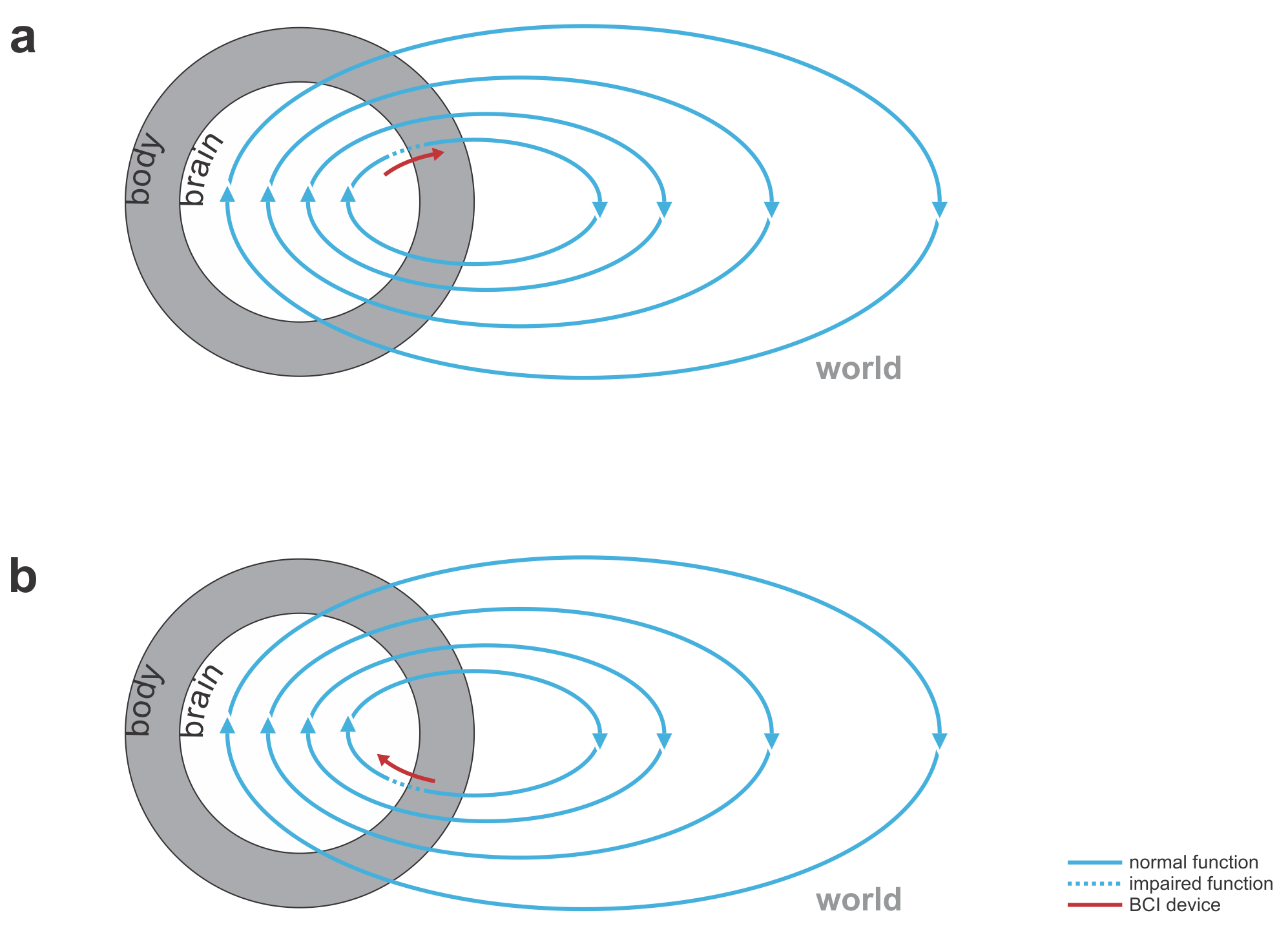
An organism in interaction with its environment forms a massively parallel perception-to-action cycle. The causal routes through the nervous system range in complexity from reflexes to higher cognition and memories at the temporal scale of the life span. The causal routes through the world, similarly, range from direct effects of our movements feeding back into our senses, to distal effects of our actions years down the line.
Any BCI must insert itself somewhere in this cycle – to supplement, or complement, some function. Typically a BCI, just like a brain, will take some input and produce some output. The input can come from the organism’s nervous system or body, or from the environment. The output, likewise, can go into the organism’s nervous system or body, or into the environment.
This immediately suggests a range of medical applications (Figs. 1, 2):
replacing lost perceptual function: The BCI’s input comes from the world (e.g. visual or auditory signals) and the output goes to the nervous system.
replacing lost motor function: The BCI’s input comes from the nervous system (e.g. recordings of motor cortical activity) and the output is a prosthetic device that can manipulate the world (Fig. 1).
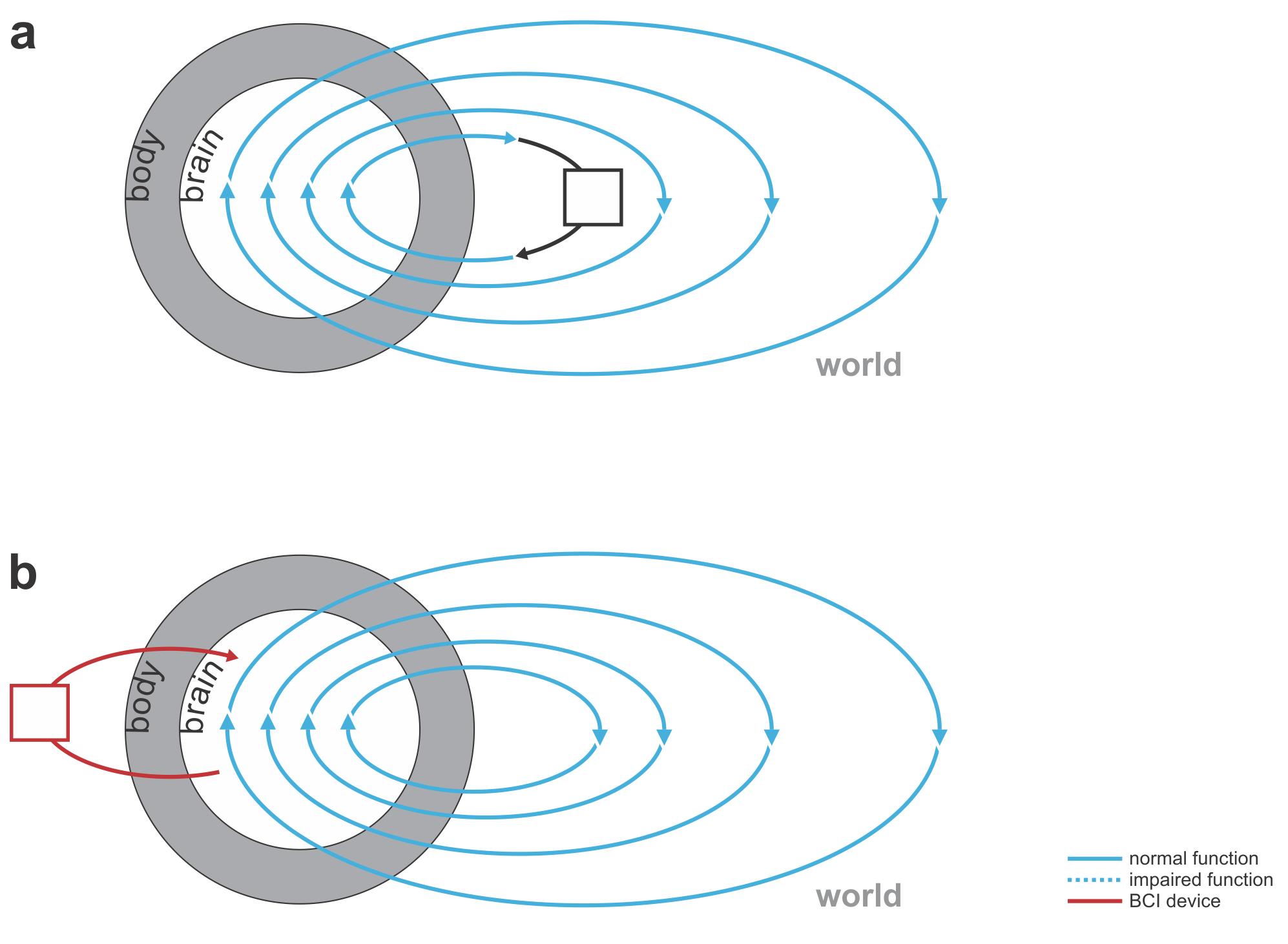
bridging lost connectivity or replacing lost nervous processing: The BCI’s input comes from the nervous system and the output is fed back into the nervous system (Fig. 2).
Fig. 1 | Uni- and bidirectional prosthetic-control BCIs. (a) A unidirectional BCI (red) for control of a prosthetic hand that reads out neural signals from motor cortex. The patient controls the hand using visual feedback (blue arrow). (b) A bidirectional BCI (red) for control of a prosthetic hand that reads out neural signals from motor cortex and feeds back tactile sensory signals acquired through artificial sensors to somatosensory cortex.
Beyond restoring lost function, BCIs have inspired visions of brain augmentation that would enable us to transcend normal function. For example, BCI’s might enable us to perceive, communicate, or act at higher bandwidth. While interesting to consider, current BCIs are far from achieving the bandwidth (bits per second) of our evolved input and output interfaces, such as our eyes and ears, our arms and legs. It’s fun to think that we might write a text in an instant with a BCI. However, what limits me in writing this open review is not my hands or the keyboard (I could use dictation instead), but the speed of my thoughts. My typing may be slower than the flight of my thoughts, but my thoughts are too slow to generate an acceptable text at the pace I can comfortably type.
But what if we could augment thought itself with a BCI? This would require the BCI to listen in to our brain activity as well as help shape and direct our thoughts. In other words, the BCI would have to be bidirectional and act as a neural co-processor (Fig. 3). The idea of such a system helping me think is science fiction for the moment, but bidirectional BCIs are a reality.
I might consider my laptop a very functional co-processor for my brain. However, it doesn’t include a BCI, because it neither reads from nor writes to my nervous system directly. It instead senses my keystrokes and sends out patterns of light, co-opting my evolved biological mechanisms for interfacing with the world: my hands and eyes, which provide a bandwidth of communication that is out of reach of current BCIs.
Fig. 2 | Bidirectional motor and sensory BCIs. (a) A bidirectional motor BCI (red) that bridges a spinal cord injury, reading signals from motor cortex and writing into efferent nerves beyond the point of injury or directly contacting the muscles. (b) A bidirectional sensory BCI that bridges a lesion along the sensory signalling pathway.
Rao reviews the exciting range of proof-of-principle demonstrations of bidirectional BCIs in the literature:
Closed-loop prosthetic control: A bidirectional BCI may read out motor cortex to control a prosthetic arm that has sensors whose signals are written back into somatosensory cortex, replacing proprioceptive signals. (Note that even a unidirectional BCI that only records activity to steer the prosthetic device will be operated in a closed loop when the patient controls it while visually observing its movement. However, a bidirectional BCI can simultaneously supplement both the output and the input, promising additional benefits.)
Reanimating paralyzed limbs: A bidirectional BCI may bridge a spinal cord injury, e.g. reading from motor cortex and writing to the efferent nerves beyond the point of injury in the spinal cord or directly to the muscles.
Restoring motor and cognitive functions: A bidirectional BCI might detect a particular brain state and then trigger stimulation is a particular region. For example, a BCI may detect the impending onset of an epileptic seizure in a human and then stimulate the focus region to prevent the seizure.
Augmenting normal brain function: A study in monkeys demonstrated that performance on a delayed-matching-to-sample task can be enhanced by reading out the CA3 representation and writing to the CA1 representation in the hippocampus (after training a machine learning model on the patterns during normal task performance). BCIs reading from and writing to brains have also been used as (currently still very inefficient) brain-to-brain communication devices among rats and humans.
Inducing plasticity and rewiring the brain: It has been demonstrated that sequential stimulation of two neural sites A and B can induce Hebbian plasticity such that the connections from A to B are strengthened. This might eventually be useful for restoration of lost connectivity.
Most BCIs use linear decoders to read out neural activity. The latent variables to be decoded might be the positions and velocities capturing the state of a prosthetic hand, for example. The neural measurements are noisy and incomplete, so it is desirable to combine the evidence over time. The system should use not only the current neural activity pattern to decode the latent variables, but also the recent history. Moreover, it should use any prior knowledge we might have about the dynamics of the latent variables. For example, the components of a prosthetic arm are inert masses. Forces upon them cause acceleration, i.e. a change of velocity, which in turn changes the positions. The physics, thus, entails smooth positional trajectories.
When the neuronal activity patterns linearly encode the latent variables, the dynamics of the latent variables is also linear, and the noise is Gaussian, then the optimal way of inferring the latent variables is called a Kalman filter. The state vector for the Kalman filter may contain the kinematic quantities whose brain representation is to be estimated (e.g. the position, velocity, and acceleration of a prosthetic hand). A dynamics model that respects the laws of physics can help constrain the inference so as to obtain more reliable estimates of the latent variables.
For a perceptual BCI, similarly, the signals from the artificial sensors might be noisy and we might have prior knowledge about the latent variables to be encoded. Encoders, as well as decoders, thus, can benefit from using models that capture relevant information about the recent input history in their internal state and use optimal inference algorithms that exploit prior knowledge about the latent dynamics. Bidirectional BCIs, as we have seen, combine neural decoders and encoders. They form the basis for a more general concept that Rao introduces: the concept of a neural co-processor.
Fig. 3 | Devices augmenting our thoughts. (a) A laptop computer (black) that interfaces with our brains through our hands and eyes (not a BCI). (b) A neural co-processor that reads out neural signals from one region of the brain and writes in signals into another region of the brain (bidirectional BCI).
The term neural co-processor shifts the focus from the interface (where brain activity is read out and/or written in) to the augmentation of information processing that the device provides. The concept further emphasizes that the device processes information along with the brain, with the goal to supplement or complement what the brain does.
The framework for neural co-processors that Rao outlines generalizes bidirectional BCI technology in several respects:
The device and the user’s brain jointly optimize a behavioral cost function:
BCIs from the earliest days have involved animals or humans learning to control some aspect of brain activity (e.g. the activity of a single neuron). Conversely, BCIs standardly employ machine learning to pick up on the patterns of brain activity that carry a particular meaning. The machine learning of patterns associated, say, with particular actions or movements is often followed by the patient learning to operate the BCI. In this sense mutual co-adaptation is already standard practice. However, the machine learning is usually limited to an initial phase. We might expect continual mutual co-adaptation (as observed in human interaction and other complex forms of communication between animals and even machines) to be ultimately required for optimal performance.
Decoding and encoding models are integrated: The decoder (which processes the neural data the device reads as its input) and encoder (which prepares the output for writing into the brain) are implemented in a single integrated model.
Recurrent neural network models replace Kalman filters: While a Kalman filter is optimal for linear systems with Gaussian noise, recurrent neural networks provide a general modeling framework for nonlinear decoding and encoding, and nonlinear dynamics.
Stochastic gradient descent is used to adjust the co-processor so as to optimize behavioral accuracy: In order to train a deep neural network model as a neural co-processor, we would like to be able to apply stochastic gradient descent. This poses two challenges: (1) We need a behavioral error signal that measures how far off the mark the combined brain-co-processor system is during behavior. (2) We need to be able to backpropagate the error derivatives. This requires that we have a mathematically specified model not only for the co-processor, but also for any further processing performed by the brain to produce the behavior whose error is to drive the learning. The brain-information processing from co-processor output to behavioral response is modeled by an emulator model. This enables us to backpropagate the error derivatives from the behavioral error measurements to the co-processor and through the co-processor. Although backpropagation proceeds through the emulator first, only the co-processor learns (as the emulator is not involved in the interaction and only serves to enable backpropagation). The emulator needs to be trained to emulate the part of the perception-to-action cycle it is meant to capture as well as possible.
The idea of neural co-processors provides an attractive unifying framework for developing devices that augment brain function in some way, based on artificial neural networks and deep learning.
Intriguingly, Rao argues that neural co-processors might also be able to restore or extend the brain’s own processing capabilities. As mentioned above, it has been demonstrated that Hebbian plasticity can be induced via stimulation. A neural co-processor might initially complement processing by performing some representational transformation for the brain. The brain might then gradually learn to predict the stimulation patterns contributed by the co-processor. The co-processor would scaffold the processing until the brain has acquired and can take over the representational transformation by itself. Whether this would actually work remains to be seen.
The framework of neural co-processors might also be relevant for basic science, where the goal is to build models of normal brain-information processing. In a basic-science context, the goal is to drive the model parameters to best predict brain activity and behavior. The error derivatives of the brain or behavioral predictions might be continuously backpropagated through a model during interactive behavior, so as to optimize the model.
Overall, this paper gives an exciting concise view of the state of the literature on bidirectional BCIs, and the concept of neural co-processors provides an inspiring way to think about the bigger picture and future directions for this technology.
Strengths
The paper is well-written and gives a brief, but precise overview of the current state of the art in bidirectional BCI technology.
The paper offers an inspiring unifying framework for understanding bidirectional BCIs as neural co-processors that suggests exciting future developments.
Weaknesses
The neural co-processor idea is not explained as intuitively and comprehensively as it could be.
The paper could give readers from other fields a better sense of quantitative benchmarks for BCIs.
Improvements to consider in revision
The text is already at a high level of quality. These are just ideas for further improvements or future extensions.
The figure about neural co-processors could be improved. In particular, the author could consider whether it might help to
clarify the direction of information flow in the brain and the two neural networks (clearly discernible arrows everywhere)
illustrate the parallelism between the preserved healthy output information flow (e.g. M1->spinal cord->muscle->hand movement) and the emulator network
illustrate the function intuitively using plausible choices of brain regions to read from (PFC? PPC?) and write to (M1? – flipping the brain?)
illustrate an intuitive example, e.g. a lesion in the brain, with function supplemented by the neural co-processor
add an external actuator to illustrate that the co-processor might directly interact with the world via motors as well as sensors
clarify the source of the error signal
The text on neural co-processors is very clear, but could be expanded by considering another example application in an additional paragraph to better illustrate the points made conceptually about the merits and generality of the approach.
The expected challenges on the path to making neural co-processors work could be discussed in more detail.
It would be good to clarify how the behavioral error signals to be backpropagated would be obtained in practice, for example, in the context of motor control.
Should we expect that it might be tractable to learn the emulator and co-processor models under realistic conditions? If so, what applied and basic science scenarios might be most promising to try first?
If the neural co-processor approach were applied to closed-loop prosthetic arm control, there would have to be two separate co-processors (motor cortex -> artificial actuators, artificial sensors -> sensory cortex) and so the emulator would need to model the brain dynamics intervening between perception and action.
It would be great to include some quantitative benchmarks (in case they exist) on the performance of current state-of-the-art BCIs (e.g. bit rate) and a bit of text that realistically assesses where we are on the continuum between proof of concept and widely useful application for some key applications. For example, I’m left wondering: What’s the current maximum bit rate of BCI motor control? How does this compare to natural motor control signals, such as eye blinks? Does a bidirectional BCI with sensory feedback improve the bit rate (despite the fact that there is already also visual feedback)?
It would be helpful to include a table of the most notable BCIs built so far, comparing them in terms of inputs, outputs, notable achievements and limitations, bit rate, and encoding and decoding models employed.
The current draft lacks a conclusion that draws the elements together into an overall view.
An elegant new study by Bracci, Kalfas & Op de Beeck (pp2018) suggests that the prominent division between animate and inanimate things in the human ventral stream’s representational space is based on a superficial analysis of visual appearance, rather than on a deeper analysis of whether the thing before us is a living thing or a lifeless object.
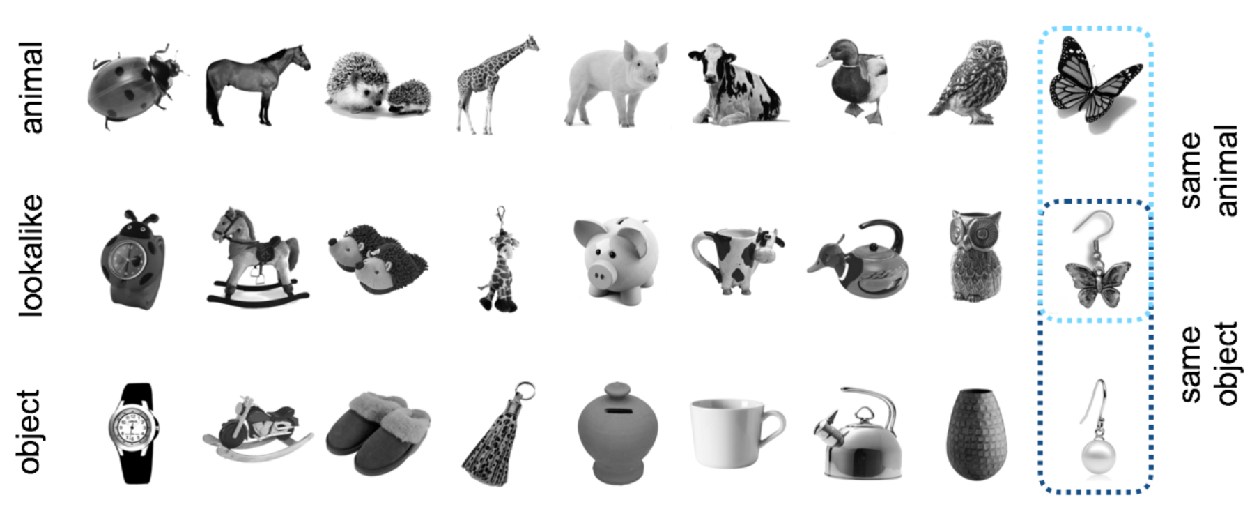
Bracci et al. assembled a beautiful set of stimuli divided into 9 equivalent triads (Figure 1). Each triad consists of an animal, a manmade object, and a kind of hybrid of the two: an artefact of the same category and function as the object, designed to resemble the animal in the triad.
Figure 1: The entire set of 9 triads = 27 stimuli. Detail from Figure 1 of the paper.
Bracci et al. measured response patterns to each of the 27 stimuli (stimulus duration: 1.5 s) using functional magnetic resonance imaging (fMRI) with blood-oxygen-level-dependent (BOLD) contrast and voxels of 3-mm width in each dimension. Sixteen subjects viewed the images in the scanner while performing each of two tasks: categorizing the images as depicting something that looks like an animal or not (task 1) and categorizing the images as depicting a real living animal or a lifeless artefact (task 2).
The authors performed representational similarity analysis, computing representational dissimilarity matrices (RDMs) using the correlation distance (1 – Pearson correlation between spatial response patterns). They averaged representational dissimilarities of the same kind (e.g. between the animal and the corresponding hybrid) across the 9 triads. To compare different kinds of representational distance, they used ANOVAs and t tests to perform inference (treating the subject variable as a random effect). They also studied the representations of the stimuli in the last fully connected layers of two deep neural networks (DNNs; VGG-19, GoogLeNet) trained to classify objects, and in human similarity judgments. For the DNNs and human judgements, they used stimulus bootstrapping (treating the stimulus variable as a random effect) to perform inference.
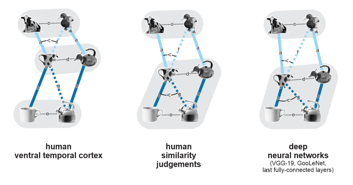
Results of a series of well-motivated analyses are summarized in Figure 2 below (not in the paper). The most striking finding is that while human judgments and DNN last-layer representations are dominated by the living/nonliving distinction, human ventral temporal cortex (VTC) appears to care more about appearance: the hybrid animal-lookalike objects, despite being lifeless artefacts, fall closer to the animals than to the objects. In addition, the authors find:
Clusters of animals, hybrids, and objects: In VTC, animals, hybrids, and objects form significantly distinct clusters (average within-cluster dissimilarity < average between-cluster dissimilarity for all three pairs of categories). In DNNs and behavioral judgments, by contrast, the hybrids and the objects do not form significantly distinct clusters (but animals form a separate cluster from hybrids and from objects).
Matching of animals to corresponding hybrids: In VTC, the distance between a hybrid animal-lookalike and the corresponding animal is significantly smaller than that between a hydrid animal-lookalike and a non-matching animal. This indicates that VTC discriminates the animals and animal-lookalikes and (at least to some extent) matches the lookalikes to the correct animals. This effect was also present in the similarity judgments and DNNs. However, the latter two similarly matched the hybrids up with their corresponding objects, which was not a significant effect in VTC.
Figure 2: A qualitative visual summary of the results. Connection lines indicate different kinds of representational dissimilarity, illustrated for two triads although estimates and tests are based on averages across all 9 triads. Gray underlays indicate clusters (average within-cluster dissimilarity < average between-cluster dissimilarity, significant). Arcs indicate significantly different representational dissimilarities. It would be great if the authors added a figure like this in the revision of the paper. However, unlike the mock-up above, it should be a quantitatively accurate multidimensional scaling (MDS, metric stress) arrangement, ideally based on unbiased crossvalidated representational dissimilarity estimates.
The effect of the categorization task on the VTC representation was subtle or absent, consistent with other recent studies (cf. Nastase et al. 2017, open review). The representation appears to be mostly stimulus driven.
The results of Bracci et al. are consistent with the idea that the ventral stream transforms images into a semantic representation by computing features that are grounded in visual appearance, but correlated with categories (Jozwik et al. 2015). VTC might be 5-10 nonlinear transformations removed from the image. While it may emphasize visual features that help with categorization, it might not be the stage where all the evidence is put together for our final assessment of what we’re looking at. VTC, thus, is fooled by these fun artefacts, and that might be what makes them so charming.
Although this interpretation is plausible enough and straightforward, I am left with some lingering thoughts to the contrary.
What if things were the other way round? Instead of DNNs judging correctly where VTC is fooled, what if VTC had a special ability that the DNNs lack: to see the analogy between the cow and the cow-mug, to map the mug onto the cow? The “visual appearance” interpretation is based on the deceptively obvious assumption that the cow-mug (for example) “looks like” a cow. One might, equally compellingly, argue that it looks like a mug: it’s glossy, it’s conical, it has a handle. VTC, then, does not fail to see the difference between the fake animal and the real animal (in fact these categories do cluster in VTC). Rather it succeeds at making the analogy, at mapping that handle onto the tail of a cow, which is perhaps an example of a cognitive feat beyond current AI.
Bracci et al.’s results are thought-provoking and the study looks set to inspire computational and empirical follow-up research that links vision to cognition and brain representations to deep neural network models.
Strengths
addresses an important question
elegant design with beautiful stimulus set
well-motivated and comprehensive analyses
interesting and thought-provoking results
two categorization tasks, promoting either the living/nonliving or the animal-appearance/non-animal appearance division
behavioral similarity judgment data
information-based searchlight mapping, providing a broader view of the effects
new data set to be shared with the community
Weaknesses
representational geometry analyses, though reasonable, are suboptimal
no detailed analyses of DNN representations (only the last fully connected layers shown, which are not expected to best model the ventral stream) or the degree to which they can explain the VTC representation
only three ROIs (V1, posterior VTC, anterior VTC)
correlation distance used to measure representational distances (making it difficult to assess which individual representational distances are significantly different from zero, which appears important here)
Suggestions for improvement
The analyses are effective and support most of the claims made. However, to push this study from good to excellent, I suggest the following improvements.
Major points
Improved representational-geometry analysis
The key representational dissimilarities needed to address the questions of this study are labeled a-g in Figure 2. It would be great to see these seven quantities estimated, tested for deviation from 0, and all 7 choose 2 = 21 pairwise comparisons tested. This would address which distinctions are significant and enable addressing all the questions with a consistent approach, rather than combining many qualitatively different statistics (including clustering index, identity index, and model RDM correlation).
With the correlation distance, this would require a split-data RDM approach, consistent with the present approach, but using the repeated response measurements to the same stimulus to estimate and remove the positive bias of the correlation-distance estimates. However, a better approach would be to use a crossvalidated distance estimator (more details below).
Multidimensional scaling (MDS) to visualize representational geometries
This study has 27 unique stimuli, a number well suited for visualization of the representational geometries by MDS. To appreciate the differences between the triads (each of which has unique features), it would be great to see an MDS of all 27 objects and perhaps also MDS arrangements of subsets, e.g. each triad or pairs of triads (so as to reduce distortions due to dimensionality reduction).
Most importantly, the key representational dissimilarities a-g can be visualized in a single MDS as shown in Figure 2 above, using two triads to illustrate the triad-averaged representational geometry (showing average within- and between-triad distances among the three types of object). The MDS could use 2 or 3 dimensions, depending on which variant better visually conveys the actual dissimilarity estimates.
Crossvalidated distance estimators
The correlation distance is not an ideal dissimilarity measure because a large correlation distance does not indicate that two stimuli are distinctly represented. If a region does not respond to either stimulus, for example, the correlation of the two patterns (due to noise) will be close to 0 and the correlation distance will be close to 1, a high value that can be mistaken as indicating a decodable stimulus pair.
Crossvalidated distances such as the linear-discriminant t value (LD-t; Kriegeskorte et al. 2007, Nili et al. 2014) or the crossnobis distance (also known as the linear discriminant contrast, LDC; Walther et al. 2016) would be preferable. Like decoding accuracy, they use crossvalidation to remove bias (due to overfitting) and indicate that the two stimuli are distinctly encoded. Unlike decoding accuracy, they are continuous and nonsaturating, which makes them more sensitive and a better way to characterize representational geometries.
Since the LD-t and the crossnobis distance estimators are symmetrically distributed about 0 under the null hypothesis (H0: response patterns drawn from the same distribution), it would be straightforward to test these distances (and averages over sets of them) for deviation from 0, treating subjects and/or stimuli as random effects, and using t tests, ANOVAs, or nonparametric alternatives. Comparing different dissimilarities or set-average dissimilarities is similarly straightforward.
Linear crossdecoding with generalization across triads
An additional analysis that would give complementary information is linear decoding of categorical divisions with generalization across stimuli. A good approach would be leave-one-triad-out linear classification of:
living versus nonliving
things that look like animals versus other things
animal-lookalikes versus other things
animals versus animal-lookalikes
animals versus objects
animal-lookalikes versus objects
This might work for devisions that do not show clustering (within dissimilarity < between dissimilarity), which would indicate linear separability in the absence of compact clusters.
For the living/nonliving destinction, for example, the linear discriminant would select responses that are not confounded by animal-like appearance (as most VTC responses seem to be), responses that distinguish living things from animal-lookalike objects. This analysis would provide a good test of the existence of such responses in VTC.
More layers of the two DNNs
To assess the hypothesis that VTC computes features that are more visual than semantic with DNNs, it would be useful to include an analysis of all the layers of each of the two DNNs, and to test whether weighted combinations of layers can explain the VTC representational geometry (cf. Khaligh-Razavi & Kriegeskorte 2014).
More ROIs
How do these effects look in V2, V4, LOC, FFA, EBA, and PPA?
Minor points
The use of the term “bias” in the abstract and main text is nonstandard and didn’t make sense to me. Bias only makes sense when we have some definition of what the absence of bias would mean. Similarly the use of “veridical” in the abstract doesn’t make sense. There is no norm against which to judge veridicality.
The polar plots are entirely unmotivated. There is no cyclic structure or even meaningful order to the the 9 triads.
“DNNs are very good, and even better than than human visual cortex, at identifying a cow-mug as being a mug — not a cow.” This is not a defensible claim for several reasons, each of which by itself suffices to invalidate this.
fMRI does not reveal all the information in cortex.
VTC is not all of visual cortex.
VTC does cluster animals separately from animal-lookalikes and from objects.
Linear readout of animacy (cross-validated across triads) might further reveal that the distinction is present (even if it is not dominant in the representational geometry.
Grammar, typos
“how an object looks like” -> ‘how an object looks” or “what an object looks like”
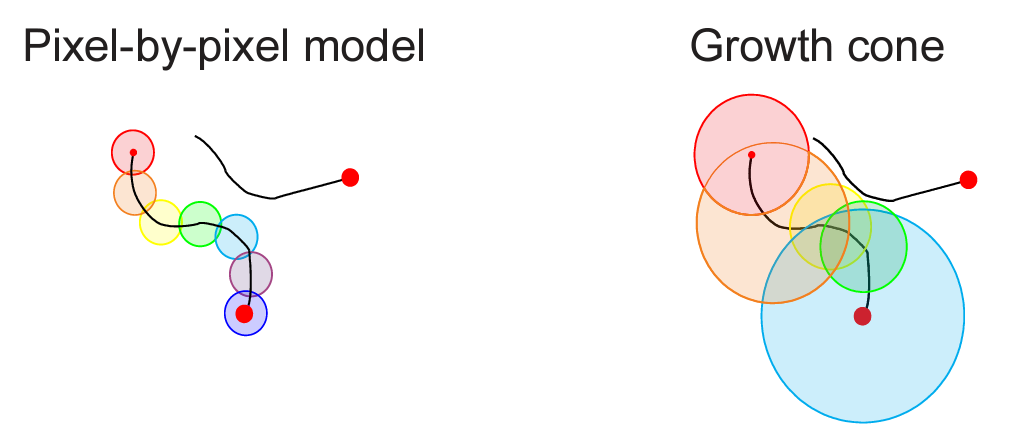
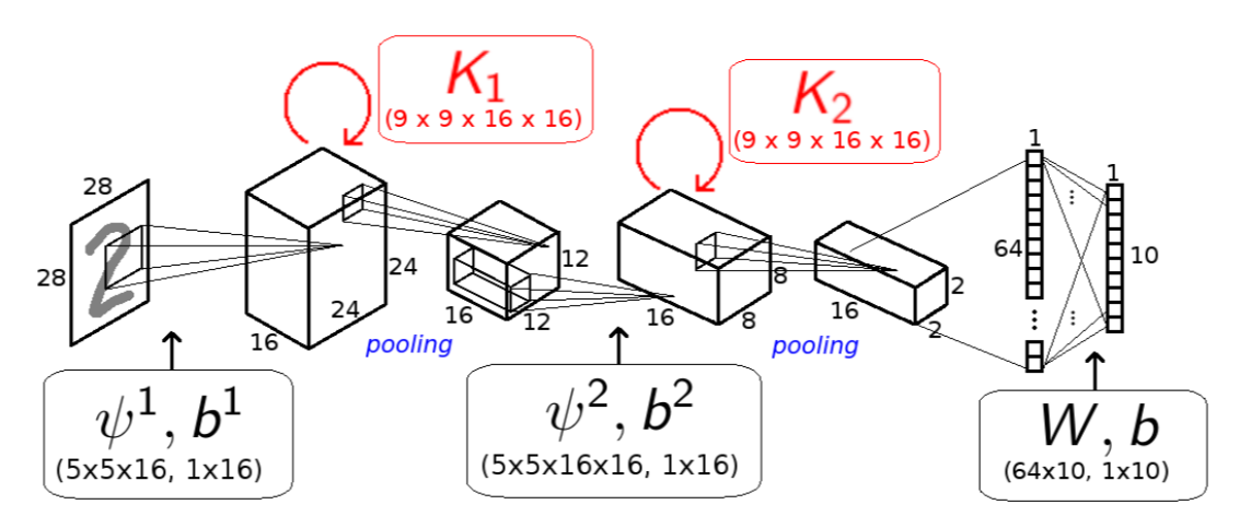
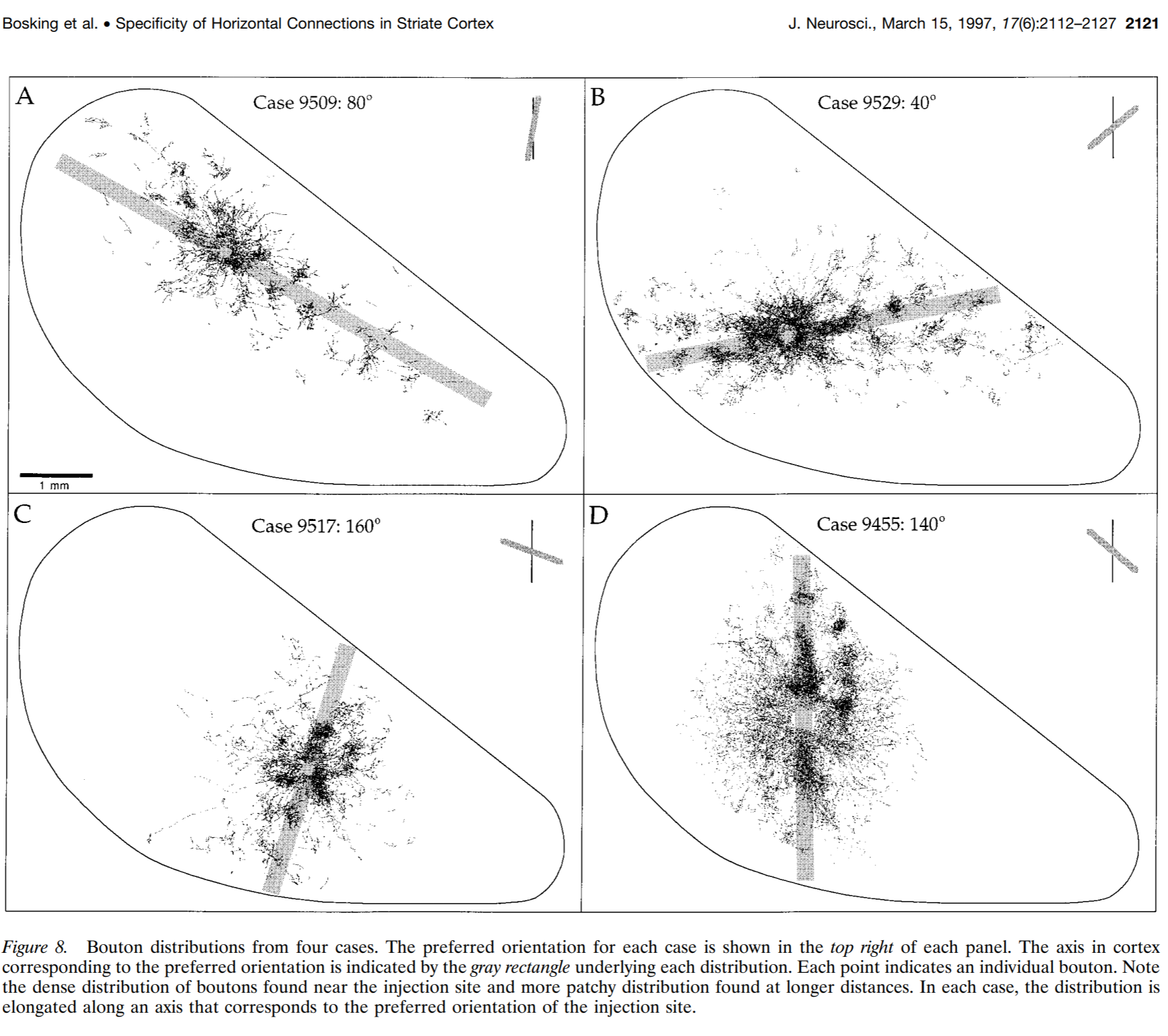
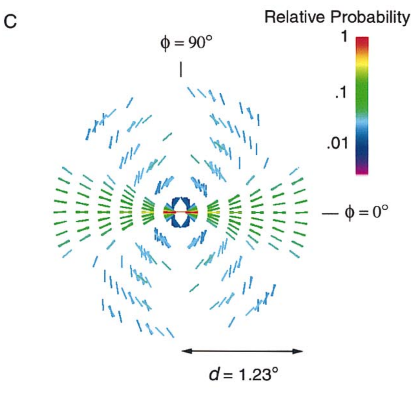
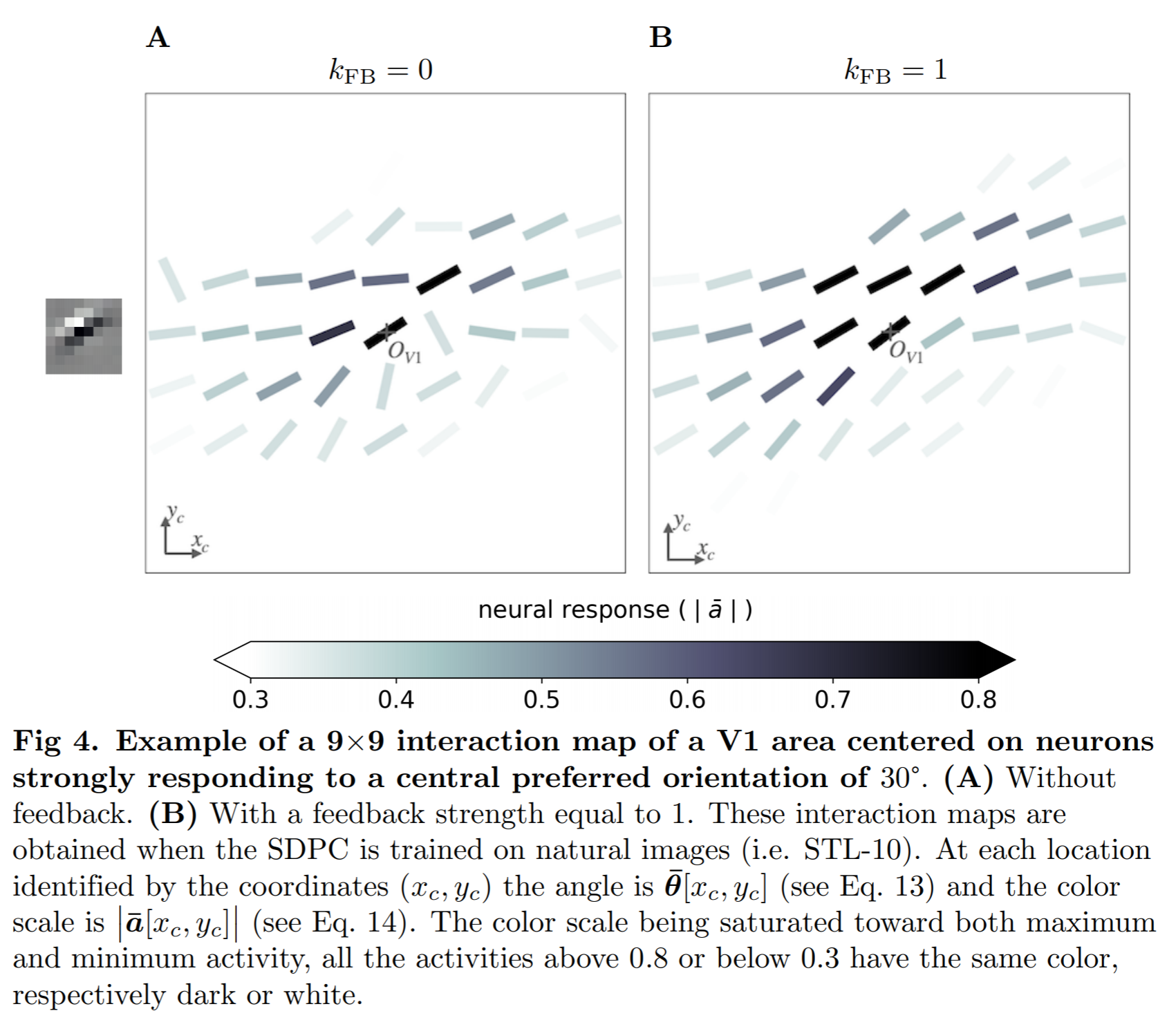
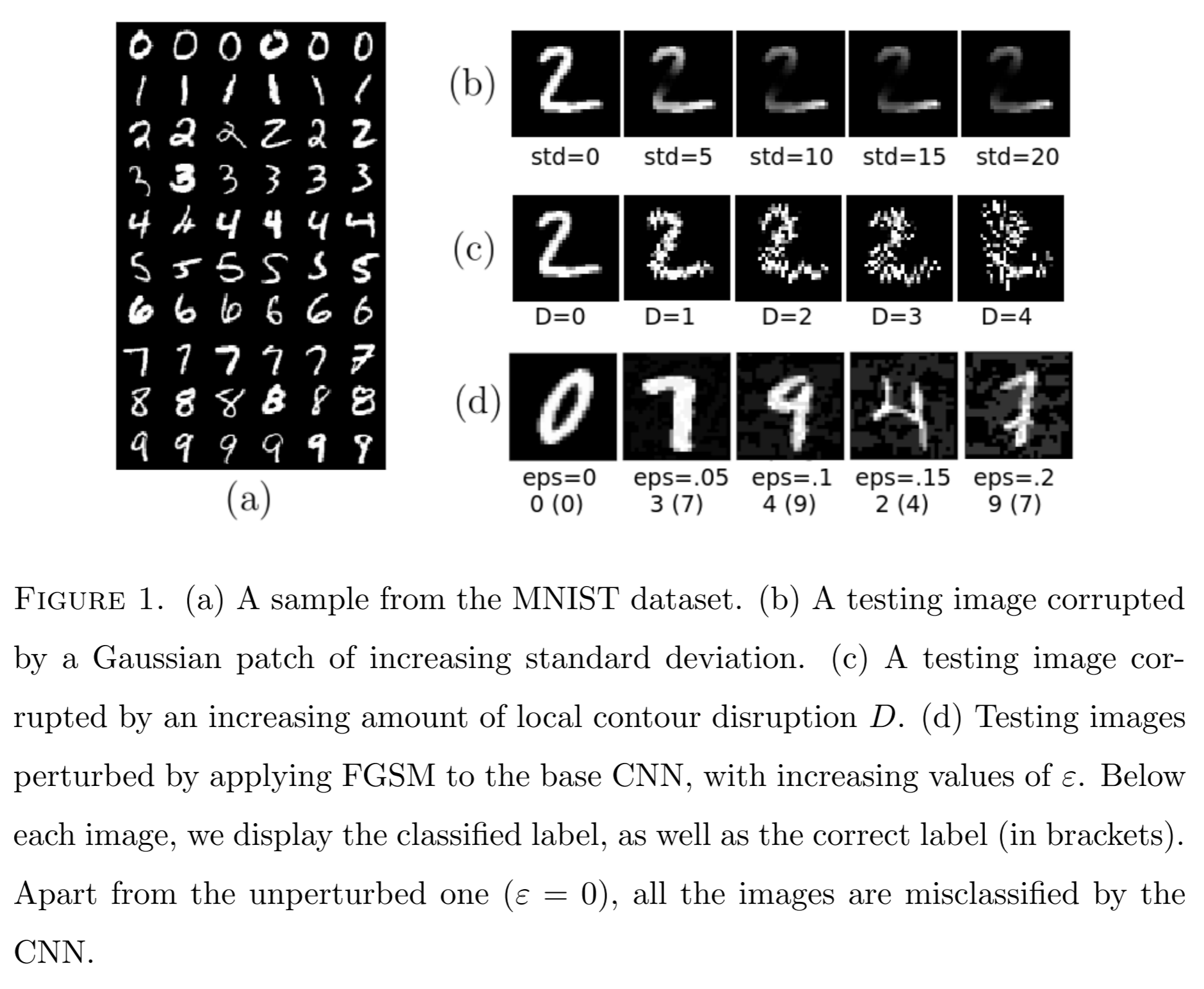
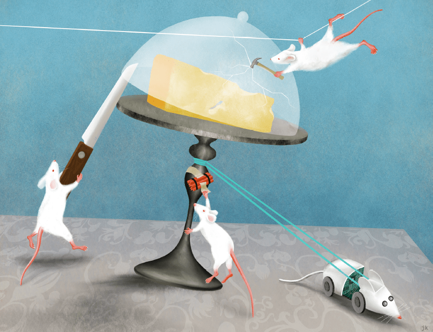
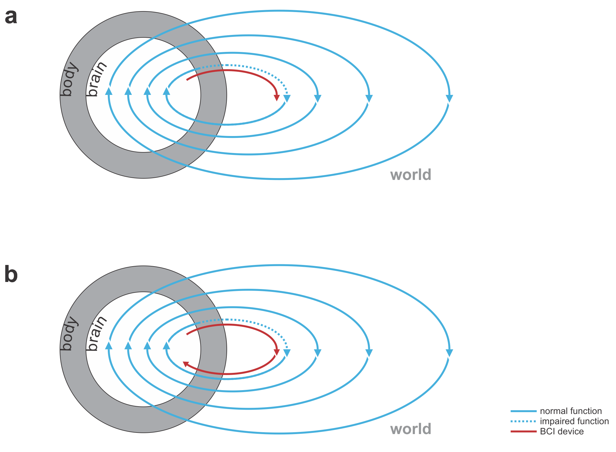 Fig. 1 | Uni- and bidirectional prosthetic-control BCIs. (a) A unidirectional BCI (red) for control of a prosthetic hand that reads out neural signals from motor cortex. The patient controls the hand using visual feedback (blue arrow). (b) A bidirectional BCI (red) for control of a prosthetic hand that reads out neural signals from motor cortex and feeds back tactile sensory signals acquired through artificial sensors to somatosensory cortex.