Tomoyasu Horikawa presents a method called “mind captioning” for decoding perceptual and cognitive content in the form of English text from human brain activity measured with functional MRI (brain-to-text: b2t). Brain-to-text decoding is an important concept because of the versatility and universality of language: It promises to enable us to read out all kinds of brain representations (not just those of linguistic content) and thus has broad potential for neuroscience and applications requiring brain-machine interfaces.
The author relied on human annotators to generate multiple verbal captions describing each of thousands of videos (video-to-text: v2t). He fed these text captions to a neural-network language model to obtain a compressed semantic feature vector characterizing the content of each video (text-to-features: t2f). He trained an L2-regularized linear decoder for each semantic feature to predict the features from human brain activity measured with functional MRI (fMRI) while subjects watched videos (brain-to-features: b2f). He then converted the features to text (features-to-text: f2t) using an iterative text synthesis procedure to invert the t2f mapping.
This iterative evolutionary text synthesis procedure is an important contribution. It proceeds from a seed (such as an uninformative token), iteratively replacing words so as to improve the correlation between the semantic feature vector predicted by the text-to-feature language model and the feature vector decoded from brain activity. The mutated captions considered are constructed by masking out particular words and then generating potential replacements using another language model (RoBERTa-large) that has been trained with masking of tokens to predict missing tokens. This masked language model provides probable completions and thus constrains the search to natural text descriptions, while the candidate descriptions best matching the decoded features are selected for further optimization.
The study also applies the decoder not only to brain activity measured while subjects view videos, but also to activity measured while subjects recall and imagine videos they previously viewed. Recall-based imagery can be decoded at levels far above chance, though much lower than perception, in high-level visual cortex. Careful encoding and decoding analyses demonstrate that information about the videos is widespread throughout the human cortex, including in the language network. However, excluding the language network for decoding did not substantially reduce decoding performance. This is a key result because the goal of brain-to-text decoding is not the decoding of verbal thoughts, but the use of text to capture the information in all kinds of brain representations, most of which are not verbal. Language is an excellent format for decoding because it can capture concrete as well as abstract information. Unlike a decoder that outputs images, a text decoder can leave out information that is unspecified in the representation being decoded.
A central claim of the study is that the results support the hypothesis that high-level visual cortex contains structured semantic representations that capture not only the sets of objects present in the scene but also their relationships (such as “man bites dog” as opposed to “dog bites man”). In addition, the author suggests that the text synthesis approach enables “faithful” decoding unbiased, or at least less biased, by prior knowledge than previous approaches (e.g. using a caption database).
Overall, this is excellent work, tackling a grand decoding challenge with many original and inspiring ideas which are expertly implemented. The analyses in the main paper and the supplementary analyses are careful and comprehensive. The examples of decoded text are impressive. However, the claim of “faithful” or “unbiased” decoding does not make sense to me. Arguably it is not even desirable to decode without prior information (i.e. without bias): To understand what the information in the brain “means”, we need to interpret it in light of what we know about the world. After all, the rest of the brain that is using the representation is also interpreting it in the context of what it knows about the world. The author should either rigorously justify these claims or leave them out.
The claims about structured semantic representation and representation of relationships may also need to be tempered a bit. I am unsure if the word shuffling analyses supporting this claim may be compromised by the fact that the resulting text is not within the distribution that the text-to-feature language model was trained on. Really addressing the structured relational semantics hypothesis would require out-of-distribution tests such as a video of a man biting a dog (an example the author introduces in the discussion), whose decoding might reveal to what extent the decoder relies on the brain representation and to what extent it infers the structure in the decoded text using its prior knowledge of the world. The paper could also be further improved by discussing the motivations for the choices made in designing the decoder and alternative choices and why they are promising or not promising.
Even if some of the claims need adjustment, this is an excellent and highly original contribution that will be of broad interest to neuroscientists and researchers in other fields.
Suggestions
Fully justify or weaken claims of “faithful” decoding unbiased by prior information.
Add a figure and table clarifying the different formats of information (video, visual features, captions, semantic features, brain activity) and all the transformations (v2t by humans, t2f by language models, b2f by linear decoder, f2t by iterative text synthesis).
Add a section to the discussion motivating the particular choices for these transformations. For example, why should brain activity and text be aligned at the level of the semantic features? Why not learn to map directly from brain activity to text? Why use an interactive inversion of the t2f model, rather than learning a direct f2t mapping? How well does the text-to-feature model preserve the information in the text? If presented with the feature vectors corresponding to a set of independent draws from the training distribution of captions (different captions, but IID), how well does the optimization method recover the description? How much of the information in the recovered verbal description is encoded in the semantic features and how much comes from the prior implicit to the text-to-feature encoder?
Add a section to the discussion addressing whether “faithful” or “unbiased” decoding is even well-defined as an ideal – whether or not it is achievable in practice.
Strengths
The paper addresses an inspiring and important challenge with scientific and applied dimensions.
Decoders are applied not only to data acquired during the viewing of videos, but also during memory-recall-driven mental imagery.
The iterative text synthesis decoding procedure is original and powerful.
The methods are original and state of the art.
The encoding and decoding analyses are comprehensive and careful, with extensive supplementary analyses and single-subject results, presenting a rich picture.
The paper uses and compares a wide range of current neural-network language models, which provide alternative semantic feature spaces.
Weaknesses
The study attempts something that may be impossible: To “faithfully” reveal the structured semantic information explicitly represented in the brain. Prior information about the language and our world inevitably informs the decoded text. It is unclear what it would even mean to decode into text without prior information.
The paper claims that the text synthesis procedure is not biased by knowledge about the world, but both the caption to semantic feature language models and the masked language model used to guide the iterative synthesis have massive knowledge of relational structure in the world that we should expect to constrain the decoded text.
The study does not include strong out-of-distribution probes of the decoders, which could reveal to what extent the relational semantic information originates from compositional brain representations or is inferred using world knowledge by the decoder.
Our retinae sample the images in our eyes discretely, conveying a million local measurements through the optic nerve to our brains. Given this piecemeal mess of signals, our brains infer the structure of the scene, giving us an almost instant sense of the geometry of the environment and of the objects and their relationships.
We see the world in terms of objects. But how our visual system defines what an object is and how it represents objects is not well understood. Two key properties thought to define what an object is in philosophy and psychology are spatiotemporal continuity and cohesion (Scholl 2007). An object can be thought of as a constellation of connected parts, such that if we were to pull on one part, the other parts would follow along, while other objects might stay put. Because the parts cohere, the region of spacetime that corresponds to an object is continuous. The decomposition of the scene into potentially movable objects is a key abstraction that enables us to perceive, not just the structure and motion of our surroundings, but also the proclivities of the objects (what might drop, collapse, or collide) and their affordances (what might be pushed, moved, taken, used as a tool, or eaten).
An important computational problem our visual system must solve, therefore, is to infer what pieces of a retinal image belong to a single object. This problem has been amply studied in humans and nonhuman primates using behavioral experiments and measurements of neural activity. A particular simplified task that has enabled highly controlled experiments is mental line tracing. A human subject or macaque fixating on a central cross is presented with a display of multiple curvy lines, one of which begins at the fixation point. The task is to judge whether a peripheral red dot is on that line or on another line (called a distractor). Behavioral experiments show that the task is easy to the extent that the target line is short or isolated from any distractors. Adding distractor lines in the vicinity of the target line to clutter up the scene and making the target line long and curvy makes the task more difficult. If the target snakes its way through complex clutter closeby, it is no longer instantly obvious where it leads and attention and time are required to judge whether the red dot is on the target or on a distractor line.
Our reaction time is longer when the red dot is farther from fixation along the target line. This suggests that the cognitive process required to make the judgment involves tracing the line with a sequential algorithm, even when fixation is maintained at the central cross. However, the reaction time is not in general linear in the distance, measured along the line, between the fixation point and the dot, as would be predicted by sequential tracing of the line at constant speed. Instead, the speed of tracing is variable depending on the presence of distracting lines in the vicinity of the current location of the tracing process along the target line. Tracing proceeds more slowly when there are distracting lines close by and more quickly when the distracting lines are far away.
The hypothesis that the primate visual system traces the line sequentially from the fixation point is supported by seminal electrophysiological experiments by Pieter Roelfsema and colleagues, which have shown that neurons in early visual cortex that represent particular pieces of the line emanating from the fixation point are upregulated in sequence, consistent with a sequential tracing process. This sequential upregulation of activity of neurons representing progressively more distal portions of the line is often interpreted as the neural correlate of attention spreading from fixation along the attended line during task performance.
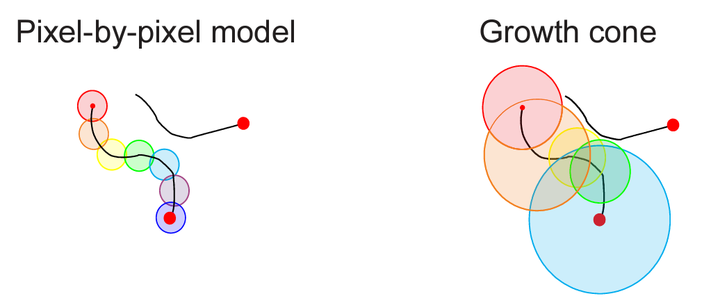
The variation in speed of the tracing process can be explained by the attentional growth-cone hypothesis (Pooresmaeili & Roelfsema 2014) which posits that attention spreads not only in the primary visual cortex but also at higher levels of cortical representation. This hypothesis can explain the variation in tracing speed: At higher levels of cortical visual representation, neurons have larger receptive fields and offer a coarser-scale summary of the image, enabling the tracing to proceed at greater speed along the line in the image. In the absence of distractors, tracing can proceed quickly at a high-level of representation. However, in the presence of distractors, the higher-level representations may not be able to resolve the scene at a sufficient grain, and tracing must proceed more slowly in lower-level representations.
Higher-level neurons are more likely to suffer from interference from distractor lines within their larger receptive fields. If a distractor line is present in a neuron’s receptive field, the neuron may not respond as strongly to the line being traced, effectively blocking the path for sequential tracing in the high-level representation. However, tracing can continue – more slowly – at lower levels, where receptive fields are small enough to discern the line without interference.
Detail from Fig. 6 in Pooresmaeili et al. (2014) illustrating the single-scale tracing model (left) and the growth-cone model (right), in which the attentional label is propagated from the fixation point (small red dot) at all levels of representation where receptive fields (circles) do not overlap with the distractor curve. Tracing proceeds rapidly at coarse scales (orange, blue) where the target line is far from the distractor and slowly at fine scales (yellow, green) where the target curve comes close to the distractor.
Now Schmid & Neumann (pp2024) offer a brain-computational model explaining in detail how this multiscale algorithm for attentional selection of the line emanating from the fixation point might be implemented in the primate brain. They describe a mechanistic model and demonstrate by simulation that it can explain how mental line tracing might be implemented in the primate brain.
Pyramidal neurons at multiple levels of the visual hierarchy (corresponding to cortical areas V1, V2, V4) detect local oriented line segments on the basis of the bottom-up signals arriving at their basal dendritic integration sites. These line segments are pieces of the target and distractor lines, represented in each area at a different scale of representation. The pyramidal neurons also receive lateral and top-down input providing contextual information at their apical dendritic integration sites, enabling them to sense whether the line segment they are representing is part of a longer continuous line.
The attentional “label” indicating that a neuron represents a piece of the target line is encoded by an upregulation of the activity of the pyramidal neurons, consistent with neural recording results from Roelfsema and colleagues (1998). The upregulation of activity, i.e. the attention label, can spread laterally within a single area such as V1. Connectivity between neurons representing approximately collinear line segments implements an inductive bias that favors interpretations conforming to the Gestalt principle of good continuation. However, the upregulation will spread only to pyramidal neurons that (1) are activated by the stimulus, (2) receive contextual input from pyramidal neurons representing approximately collinear line segments, and (3) receive thalamic input indicating the local presence of the attentional marker.
Each step of propagation is conditioned on the conjunction of these three criteria. The neural computations could be implemented exploiting the intracellular dynamics in layer-5 pyramidal neurons, where dendritic inputs entering at apical integration sites cannot drive a response by themselves but can modulate responses to inputs entering at basal integration sites. An influential theory suggests that contextual inputs arriving at the apical dendritic integration sites modulate the response to bottom-up stimulus inputs arriving at the basal dendritic integration sites (Larkum 2013, BrainInspired podcast). Schmid and Neumann’s model further posits that the apical inputs are gated by thalamic inputs (Halassa & Kastner 2017), implementing a test of the third criterion for propagation of the attentional label.
The attentional label is propagated locally from already labeled pyramidal neurons to pyramidal neurons at all levels of the visual hierarchy that represent closeby line segments sufficiently aligned in orientation to be consistent with their being part of the target line. To enable the coarser-scale representations in higher cortical areas to speed the process, neurons representing the same patch of the visual field at different scales are connected through thalamocortical loops. Through the thalamus, each level is connected to all other levels, enabling label propagation to bypass the stages of the hierarchy. The thalamic component (possibly in the pulvinar region of the visual thalamus) represents a map of the labeled locations, but not detailed orientation information.
Imagine a mechanical analogy, in which tube elements represent local segments of the lines. The stimulus-driven bottom-up signals align the orientations of the tube elements with the orientations of the line segments they represent, so the tube elements turn to form long continuous tunnels depicting the lines. A viscous liquid is injected into the tube element representing the fixation point and spreads. Adjacent tube elements need to be aligned for the liquid to flow from one into the other. In addition, there are valves between the tube elements, which open only in the presence of thalamic input. Importantly, the viscous liquid can flow not only at the V1 level of representation, where the tube elements represent tiny pieces of the lines and the viscous liquid needs to flow through many elements to reach the end of the line. Rather, the liquid can also take shortcuts through higher-level representations, where long stretches of the line are represented by few tube elements. This enables the liquid to reach the end of the line much more quickly – to the extent that there are stretches sufficiently isolated from the distractors for coarse-scale representation at higher levels of the hierarchy.
Since the information about (1) the presence of oriented line segments, (2) their compatibility according to the Gestalt principle of good continuation, and (3) the attentional label are all available in the cortical hierarchy, a growth-cone algorithm could be implemented without thalamocortical loops. However, Schmid and Neumann argue that the non-orientation-specific thalamic representation reduces the complexity of the circuit. Fewer connections are required by decomposing the question “Are there upregulated compatible signals in the neighborhood?” into two simpler questions: “Are there compatible signals in the neighborhood?” (answered by cortex) and “Are there upregulated signals in the neighborhood?” (answered by the thalamic input). Because there could be compatible signals in the neighborhood that are not upregulated, and upregulated signals that are not compatible, yeses to both questions of the decomposition do not in general imply a yes to the original question. However, if we assume that there is only one line segment per location, then two yeses do imply a yes to the original question.
Schmid and Neumann argue that thalamic label map enables a simpler circuit that works in the simulations presented, even tracing a line as it crosses another line without spillover. We wonder if, in addition to requiring fewer connections, the thalamic label map might have functional advantages in the context of a system that must be able to perform not just line tracing but many other binding tasks, where the thalamus might have the same role, but the priors defining compatibility could differ.
Why is this model important? Line tracing is a type of computational problem that is prototypical of vision and yet challenging for both of our favorite modes of thinking about visual computations: deep feedforward neural networks and probabilistic inference. These two approaches (discriminative and generative to a first approximation) form diametrically opposed corners in a vast space of visual algorithms that has only begun to be explored (Peters et al. pp2023). Line tracing is a simple example of a visual cognition task that can be rendered intractable for both approaches by making the line snaking its way through the clutter sufficiently long and the clutter sufficiently close and confusing. Feedforward deep neural networks have trouble with this kind of problem because there are no hints in the local texture revealing the long-range connectivity of the lines. The combinatorics creates too rich a space of possible curves to represent with a hierarchy of features in a neural network. Although any recurrent computation (including the model of Schmid and Neumann and a recent line tracing model from Linsley & Serre, 2019) can be unfolded into a feedforward computational graph, the feedforward network would have to be very deep, and its parameters might be hard to learn without the inductive bias that iterating the same local propagation rule is the solution to the puzzle (van Bergen & Kriegeskorte 2020). From a probabilistic inference perspective, similarly, the problem is likely intractable in its general form because of the exponential number of possible groupings we would need to compute a posterior distribution over.
By assuming that we can be certain about the way things connect locally, we can avoid having to maintain a probability distribution over all possible line continuations from the fixation point. Binarizing the probabilities turns the problem into a region growing (or graph search) problem requiring a sequential procedure, because later steps depend on the result of earlier steps.
Schmid and Neumann’s paper describes how the previously proposed growth-cone algorithm, which solves an important computational challenge at the heart of visual cognition (Roelfsema 2006), might be implemented in the primate brain. The paper seriously engages both the neuroscience (at least at a qualitative level) and the computational problem, and it connects the two. The authors simulate the model and demonstrate its predictions of the key behavioral and neurophysiological results from the literature. They use model-ablation experiments to establish the necessity of different components. They also describe the model at a more abstract level: reducing the operations to sequential logical operations and systematically considering different possible implementations in a circuit and their costs in terms of connections. This resource-cost perspective deepens our understanding of the algorithm and reveals that the proposed model is attractive not only for its consistency with neuroanatomical, neurophysiological, and behavioral data, but also for the efficiency of implementation in a physical network.
Strengths
Offers a candidate explanation for how an important cognitive function might be implemented in the primate brain, using an algorithm that combines parallel computation, hierarchical abstraction, and sequential inference.
Motivated by a large body of experimental evidence from neurophysiological and behavioral experiments, the model is consistent with primate neuroanatomy, neural connectivity, neurophysiology, and subcellular dynamics in multi-compartment pyramidal neurons.
Describes a class of related algorithms and network implementations at an abstract level, providing a deeper understanding of alternative possible neural mechanisms that could perform this cognitive function and their network complexity.
Weaknesses
The model operates on a toy version of the task, using abstracted stimuli with few orientations and predefined Gabor filter banks as model representations, rather than more general visual representations learned from natural images. An important question is to what extent the algorithm will be able to perform visual tasks on natural images. Given the complexity of the paper as is, this question should be considered beyond the scope, but related work connecting these ideas to computer vision could be discussed in more detail.
Major suggestions
(1) Illustrate the computational mechanism and operation of the model more intuitively. In Fig. 1b, colors code for the level of representations. It would therefore be better to not use green to code for the selection tag. Thicker black contours or some other non-color marker could be used. It is also hard to see that the no-interference and the interference cases have different stimuli. Only the bottom panels with the stimuli show a slight difference. The top panels should be distinct as well since different neurons would be driven by the two stimuli. Alternatively, you could consider using only one stimulus, where the distractor distance variation is quite pronounced, but showing time frames to illustrate the variation of the speed of the progression of attentional tagging.
(2) Discuss challenges in scaling and calibrating the model for application to natural continuous curves. The stimuli analyzed have only a few orientations with sudden transitions from one to the other. Would the model as implemented also work for continuous curves such as those used in the neurophysiological and behavioral experiments or would a finer tiling of orientations be required? Under what conditions would attention spill over to nearby distractor curves? It would be good to elaborate on the roles of surround suppression, inhibition among detectors, and the excitation/inhibition balance.
(3) Discuss challenges in scaling the model to computer vision tasks on natural images. To be viable as brain-computational theories, models ultimately need to scale to natural tasks. Please address the challenges of extending the model for application to natural images and computer-vision tasks. This will likely require the representations to be learned through backpropagation. The cited complementary work by Linsley and Serre on the pathfinder task using horizontal gated recurrent units and incremental segmentation for computer vision is relevant here and deserves to be elaborated on in the Discussion. In particular, do the growth-cone model and your modeling results suggest an alternative neural network architecture for learning incremental binding operations?
Minor suggestions
(1) Please make sure that the methods section contains all the details of the model architecture needed for replication of the work. Much of the math is described well. But some additional technical details on maps and connectivity may be needed. What are the sizes of the maps? What do they look like for a given input? Do they appear like association fields? What is the excitatory and inhibitory connectivity as a function of spatial locations and orientations of the source and target unit?
(2) Discuss how the model relates to the results of Chen et al. (2014) who described the interplay between V1 and V4 during incremental contour integration on the basis of simultaneous recordings in monkeys.
(3) Although the paper is well-written and clear, the English is a bit rocky throughout with many grammatical errors and some typos. These could be fixed using a proofreader or suitable software.
– Nikolaus Kriegeskorte & Hossein Adeli
References
Chen M, Yan Y, Gong X, Gilbert CD, Liang H, Li W (2014) Incremental integration of global contours through interplay between visual cortical areasNeuron.
Halassa MM, Kastner S. Thalamic functions in distributed cognitive control. Nature neuroscience. 2017 Dec;20(12):1669-79.
Lamme VA, Roelfsema PR (2000) The distinct modes of vision offered by feedforward and recurrent processingTrends in Neurosciences.
Larkum M. A cellular mechanism for cortical associations: an organizing principle for the cerebral cortex. Trends in neurosciences. 2013 Mar 1;36(3):141-51.
Larkum ME, Zhu JJ, Sakmann B (1998) A new cellular mechanism for coupling inputs arriving at different cortical layers Nature.
Linsley D, Kim J, Veerabadran V, Serre T (2019) Learning long-range spatial dependencies with horizontal gated-recurrent unitsNeurIPS. arxiv.org/abs/1805.08315.
Peters B, Kriegeskorte N (2021) Capturing the objects of vision with neural networks. Nature human behaviourNature Human Behavior.
Peters B, DiCarlo JJ, Gureckis T, Haefner R, Isik L, Tenenbaum J, Konkle T, Naselaris T, Stachenfeld K, Tavares Z, Tsao D, Yildirim I, Kriegeskorte N (under review) How does the primate brain combine generative and discriminative computations in vision? CCN GAC paper. arXiv preprint arXiv:2401.06005.
Pooresmaeili A, Roelfsema PR (2014) A growth-cone model for the spread of object-based attention during contour groupingCurrent Biology.
Roelfsema PR, Lamme VA, Spekreijse H (1998) Object-based attention in the primary visual cortex of the macaque monkeyNature.
Roelfsema PR (2006) Cortical algorithms for perceptual groupingAnnu Rev Neurosci.
Scholl BJ (2007) Object persistence in philosophy and psychologyMind & Language.
van Bergen RS, Kriegeskorte N (2020) Going in circles is the way forward: the role of recurrence in visual inferenceCurrent Opinion in Neurobiology.
Neural network (NN) models have brought spectacular progress in computer vision and visual computational neuroscience over the past decade, but their performance, until recently, was quite brittle: breaking down when images are compromised by occlusions, lack of focus, distortions, and noise — sources of nuisance variation that human vision is robust to. The robustness of recognition has substantially improved in recent models with extensive training and data augmentation.
Extensive visual experience also drives the development of human visual abilities. Humans, too, experience a vast number of visual impressions, many of them compromised and all of them embedded in a context of previous visual impressions and information from other sensory modalities, including audition, that can constrain the interpretation of the scene and drive visual learning. Do state-of-the-art robust NN models provide a good model of robust recognition in humans, then?
A new paper by Huber et al. (pp2022) suggests that a training-based account of the robustness of human vision, along the lines of the recent advances in getting NN models to be more robust through extensive training, is uncompelling. Current NN models, they argue, lack some essential computational mechanisms that enables the human brain to achieve robustness with less visual experience.
The authors measured recognition abilities in 146 children and adolescents, aged 4-15, and found that even the 4-6 year-olds outperformed current NN models at recognizing images robustly under substantial local distortions (so called eidolon distortions). They argue that back-of-the-envelope estimates of the amount of visual experience suggest that humans achieve greater robustness with less training data. The human visual system must have some additional mechanism in place that current NN models lack.
One possibility is that human vision has mechanisms to perceive the global shape of objects more robustly than current NN models. Using ingenious shape-texture-cue-conflict stimuli, which they introduced in earlier work, the authors show that the well-known human bias in favor of classifying objects by their shape is already present in the 4-6 year olds. Testing the models with the shape-texture-cue-conflict stimuli showed, by contrast, that even the most extensively trained and robust NN models rely much more strongly on texture than on shape.
To compare the amount of visual experience between humans and models, the authors offer a back-of-the-envelope calculation (their appropriate term), in which they quantify human visual experience at a given age in the currency of NN models: number of images. They use estimates of the number of waking hours across childhood and of the number of fixations per second. One fixation is assumed as roughly equivalent to a training image. According to such estimates, the best model (SWAG) requires about an order of magnitude more data to reach human-level robustness.
This calculation and the corresponding figure are interesting because they provide a starting point for an important discussion. However, the estimate suggesting an order of magnitude difference in the amount of data required could easily be off by more than an order of magnitude.
More importantly, the estimate (though it is an interesting starting point) is fundamentally flawed and should be accompanied by more critical arguments. Human visual experience is temporally continuous and dependent and therefore cannot meaningfully be quantified in terms of a number of training images or exposures (counting multiple exposures to augmented versions of the same image across epochs).
It is also unclear why fixations should be equated to images. We see a dynamic world evolve at a rate much faster than the rate of fixations. Moreover, fixations are actively chosen, so their information content may be greater than that of a similar number of i.i.d. samples. (This could count as one of the qualitative differences between primate vision and current NN models: Primate visual recognition is active perception, and visual learning is active learning: The animal makes its own curriculum and this could contribute to its learning more from less data.)
A simpler calculation (and the one I couldn’t resist typing into my calculator before getting to the authors’) would equate frames (perhaps 10 per second?) to training images. Of course, frames are not a well-defined concept, either, in the context of human visual experience and, at 10 frames per second, successive frames are highly dependent. However, temporal dependency may be a critical feature, helping rather than hurting visual learning. At 10 frames per second, the calculation yields an estimate surprisingly close to the “amount of visual experience” of the state-of-the-art models.
Another reason why comparing visual experience between models and humans is inherently difficult concerns the quality, rather than the quantity, of the visual input. The out-of-distribution generalization challenge is not (and cannot readily be) matched between humans and models. Human visual experience may include more distorted inputs due to physical processes in the world such as rain and glass obscuring the scene as well as due to optical imperfections of our eyes. As a result, human visual experience may provide better training for generalizing to the eidolon distortions than the training sets used for the most extensively trained models (SWAG and SWSL).
The claims relating to the comparison of the “amount of visual experience” between humans and models should be tempered in revision and more critically discussed with a view to directions for future studies. It would also be good to add statistical inference to demonstrate that the reported effects generalize across stimuli and subjects. The error consistency analysis is important. However, I find the boxplots hard to interpret. It would be great to see inferential comparisons between different DNNs, where currently DNNs are lumped together despite the fact that there appears to be little inter-DNN error consistency.
The authors are almost certainly correct that current NN models lack essential computational mechanisms. However, I’m not sure if the estimates of the amount of visual experience in the current version of the paper provide strong evidence for the greater data efficiency of human vision.
Overall this paper describes an important, carefully designed and executed study and offers a unique open-science human developmental cross-sectional data set on object-recognition robustness for further systematic analyses. The use of state-of-the-art models and the careful discussion of the state of the field make this a great contribution.
Strengths
Important comprehensive novel behavioral data set
Challenge of experimenting with kids of different ages met with carefully designed and executed experiment
All code and data available via github
Comparison to four NN models that represent the state of the art at out-of-distribution robust recognition and span four orders of magnitude of training-set size (1M, 10M, 100M, 1B images)
Interesting discussion highlighting the difficulty of quantifying and comparing “the amount of visual experience” between models and humans
Weaknesses
The “back-of-the-envelope” calculation on the amount of visual experience is not just a very rough approximation, but conceptually flawed: Human visual experience is temporally continuous and dependent, and thus cannot be approximately quantified in terms of a number of i.i.d. images.
The out-of-distribution generalization challenge is not (and cannot readily be) matched between humans and models. Human visual experience may provide better training for generalizing to the eidolon distortions than the training sets used for the most extensively trained models (SWAG and SWSL).
Hypotheses are not evaluated by statistical inference to generalize to the populations of subjects and stimuli.
Age may be confounded by ability to attend on the task and by factors related to participant recruitment. (However, this reflects inherent difficulties of the research not shortcomings of this particular study.)
Model architecture is not varied systematically and independently of training regime. (However, this is very hard to achieve given the scale of the models and training sets, and they key conclusions appear compelling despite this shortcoming.)
Minor notes
“not only subjective effortless but objectively often impressive” typo: should be “subjectively”. Also: impressiveness is inherently subjective.
knive -> knife
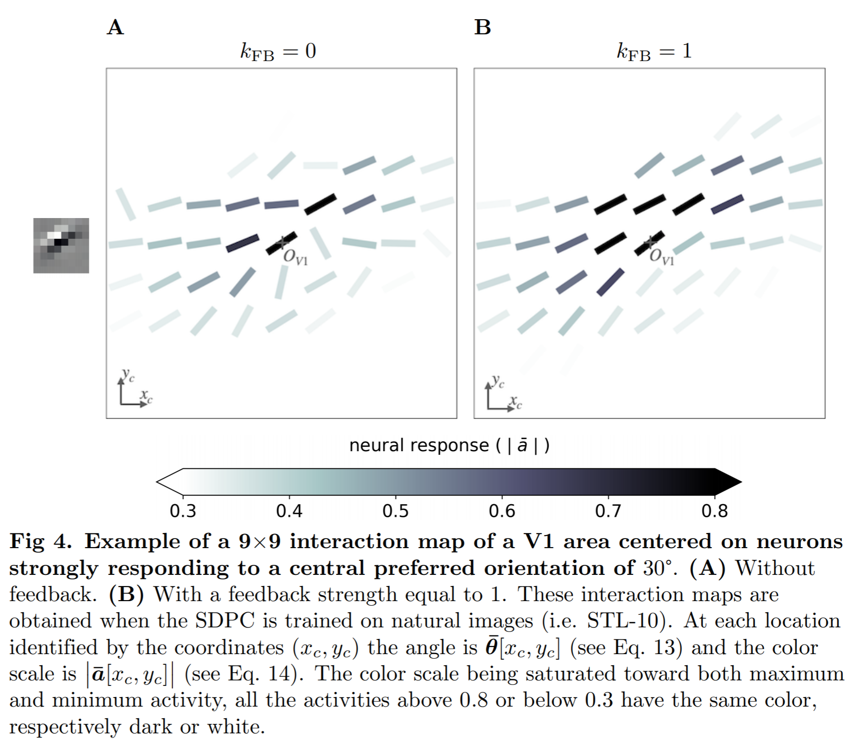
Fig. 4: Panel labels (a), (b) should be bigger, bold and above, not below the panels. The top should be a.
Fig. 4a: The logarithmic horizontal axis tick labels are inconsistent between the panels.
Fig. 5 (left): accuracy delta should be described “4-6 year-olds minus adults”, not vice versa
Proprioception is our sense of the motion and posture of our own body. This sixth sense uses signals from receptors in the joints, tendons, muscles, and skin that measure forces and degrees of extension. These receptors enable us to sense, for example, the posture of our body as we wake from sleep. They also provide feedback signals that help us precisely control our limbs, for example during handwriting.
Feedback is thought to be essential to motor control, enabling the controller in our brains to rapidly adapt to the unexpected. The unexpected may include changes in the environment (like something pushing our hand that we didn’t see coming), changes in our bodies (such as muscle fatigue or injury), and shortcomings of the motor program (such as a lack of precision or a badly planned limb trajectory). Feedback can come from vision and even audition, but proprioception provides an essential additional feedback path that informs us directly about the motion and posture of our limbs, and any forces on them.
How does feedback control work in the human motor system? I want to write a ‘k’, but there are forces on my limbs resulting from the friction of chalk on this particular blackboard. Also, my muscles are recovering from tennis practice this morning, and I haven’t used chalk on a blackboard in years.
If the goal is to write a ‘k’, I have some flexibility. I am committed, not to a precise trajectory, but to a more abstractly defined objective: to write a legible ‘k’. This suggests that feedback processing should evaluate to what extent I am succeeding at the action, not at tracing out a particular trajectory. Does what I’m actually doing look like writing a ‘k’?
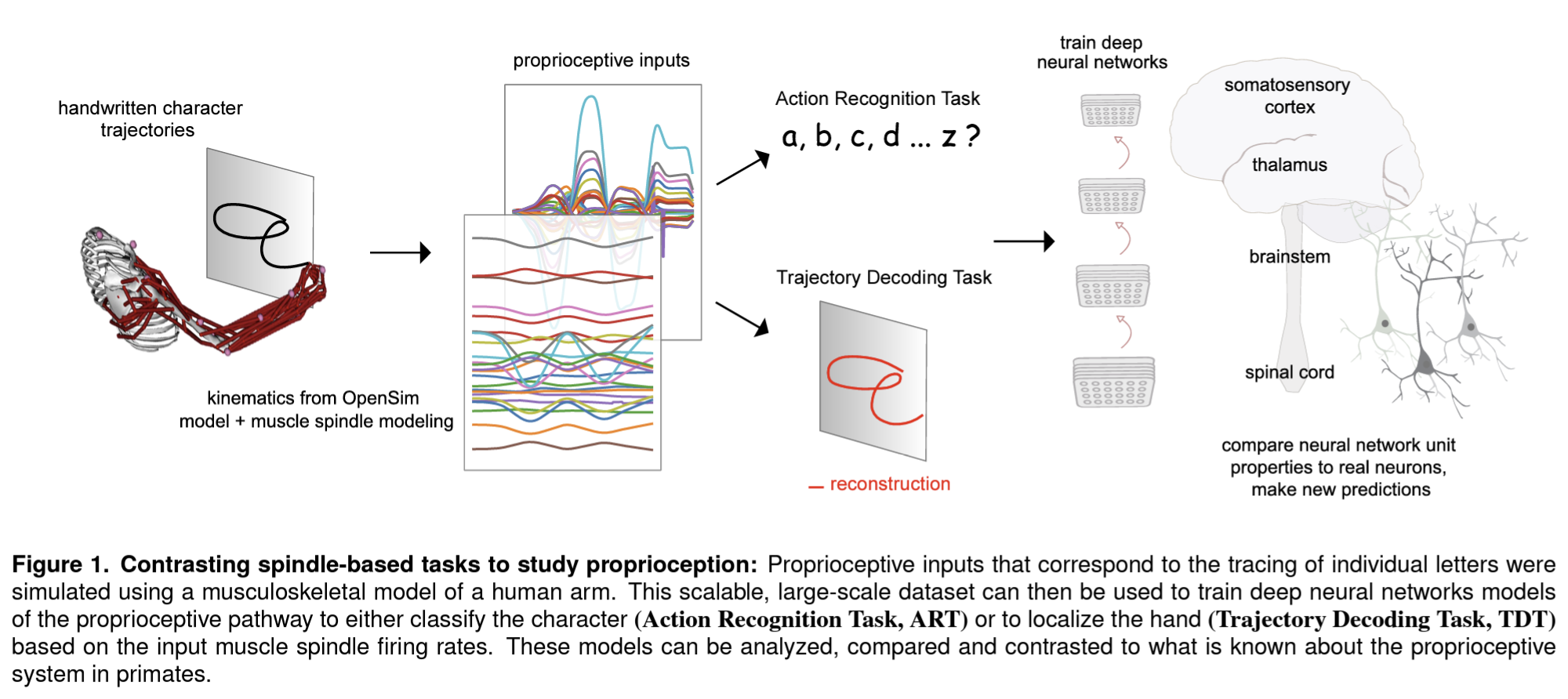
In a new paper, Sandbrink et al. (pp2022) report on simulations of the human musculoskeletal system and neural network models that suggest that the tuning properties of neurons in somatosensory cortex (S1) can be explained by assuming that the objective of the proprioceptive system is to recognize the action being performed.
They used recorded traces of a person writing lower-case letters to simulate the responses of muscle spindles sensing the lengths and velocities of muscles in the human arm as would be present if the hand were moved passively along these trajectories. The physical simulation uses a 3D model of the human arm with two parameters for the direction of the upper arm and two more for the direction of the lower arm. These four parameters are inferred by inverse kinematics from the hand trajectories tracing each letter in a variety of vertical and horizontal planes. A 3D muscle model then enables the authors to compute the expected spindle responses that reflect the lengths and velocities of 25 relevant upper arm muscles.
The authors then trained neural network models of proprioceptive processing that took the simulated muscle spindle signals as input. The neural net architectures included one that first integrates information over the muscle spindles and then across time (“spatial-temporal”), one that integrated across muscle spindles and time simultaneously (“spatiotemporal”), and a recurrent long-short-term-memory model.
Each architecture was trained on two objectives: to decode the trajectory (i.e. the position of the hand tracing a letter as a function of time) or to recognize the action (i.e. the letter being traced). The two objectives correspond to two hypotheses about the function of proprioceptive processing: To inform the feedback controller about either the current position of the hand or the letter being drawn.
The models trained to recognize the action developed tuning more consistent with what is known about the tuning of neurons in primary somatosensory cortex in primates. In particular, direction tuning with roughly equal numbers of units preferring each direction emerged in middle layers of the neural network models trained to recognize the action, similar to what has been observed in primate neural recordings. Direction tuning is already present in the muscle-spindle signals, but the spindle signals do not uniformly represent the directions.
The task-optimization approach to neural network modeling is inspired by work in vision, where neural networks trained on the task of image classification explained responses to novel images in populations of neurons in the inferior temporal cortex. This result suggested a tentative answer to the why question: Why do inferior temporal neurons exhibit the response profiles and representational geometry they exhibit? Because their function (or one of their functions) is to recognize the objects in the images. Here, similarly, the authors address a why question with task-optimized neural network models: Why do somatosensory cortical neurons exhibit the types of tuning that have been reported in the literature?
The function of proprioception, of course, is not for the brain to recognize which letter it is trying to write. It already knows that. The function is to sense how the current trajectory – the actual, not the intended one – differs from, say, a legible “k” (if that was the intention), and to map from that difference to a modification vector that will improve the outcome.
Why is action decoding relevant for performing the action? A key reason may be that the goal is not to produce a fixed trajectory, but to produce a legible ‘k’. A legible ‘k’ is not a single trajectory, but a class of trajectories containing an infinity of viable solutions. If someone nudged my arm while writing, adaptive feedback control should not attempt to return me to the originally intended trajectory, but to a new trajectory that traces the most legible ‘k’ that is still in the cards, which may be a different style of ‘k’ than I originally intended.
The paper contributes a useful data set for training models and a qualitative comparison of models to real neurons in terms of tuning properties. It would be good, in follow-up studies, to directly test to what extent each of the models can quantitatively predict either single-neuron responses or population representational geometries, as has been done in vision, and to perform statistical comparisons between models.
Importantly, this paper develops the idea of combining simulations body and brain, of the musculoskeletal system and the processing of control-related signals in the nervous system, which provides a very exciting direction for future research.
Strengths
The paper introduces a highly original research program that marries simulation of the musculoskeletal system and neural network modelling to predict neural representations in the proprioceptive pathway.
The authors performed an architecture search and trained multiple instances of different neural network architectures with each of two objectives.
The paper includes comprehensive analyses of the proprioceptive representations from the simulated muscle-spindle signals through the layers of the models. These analyses characterize unit tuning, linear decodability, and representational similarity.
The results suggest an explanation for the direction tuning with a roughly uniform distribution of the units’ direction preferences that has been reported previously for neurons in the primate primary somatosensory (S1) cortex.
If the simulated muscle-spindle data set, models, and analysis code were shared along with the published paper, this work could form the basis for quantitative model evaluation and further model development.
Weaknesses
The models are qualitatively evaluated by comparison of model unit tuning to what is known about the tuning of neurons in somatosensory cortex. Follow-up studies should quantitatively evaluate the models by inferential analyses of their ability to predict measured responses.
The two training objectives differ in multiple respects, making it difficult to assess what the necessary requirements are for the emergence of representations similar to primate S1. Decoding the hand position may be too simple, but what about decoding velocity, or trajectory descriptors such as curvature? There may be a middle ground between trajectory decoding and action recognition that also leads to the emergence of tuning properties as found in primate S1.
The authors usefully define the term mapping model in contradistinction to models of brain function. A mapping model specifies the mapping between a model of brain function (some brain-representational model) and brain-activity measurements. A mapping model can relate brain-activity measurements to different types of brain-representational model: (1) descriptions of the stimuli, (2) descriptions of behavioral responses, (3) activity measurements in other brains or other brain regions, or (4) the units in some layer of a neural network model. Moreover, mapping models can operate in either direction: from the measured brain activity to the features of the representational model (decoding model) or from the model features to the measured brain activity (encoding model). Figures 1 and 2 of the paper very clearly lay out these important distinctions.
To begin addressing the question what mapping models should be used the authors consider three desiderata: (1) predictive accuracy, (2) interpretability, and (3) biological plausibility. Predictive accuracy tends to favor more complex and nonlinear models (assuming we have enough data for fitting), whereas simpler and linear models may be easier to interpret in general. Biological plausibility would appear to be irrelevant if the mapping model is not considered a model of brain function. However, in the context of an encoding model, for example, we may want the mapping model to capture physiological processes such as the hemodynamics and nonphysiological processes such as the averaging in voxels, neither of which may be considered part of the brain-computational process that is the ultimate target of our investigation.
The authors make many reasonable points about linear and nonlinear mapping models and conclude by suggesting that rather than the linear/nonlinear distinction, we should consider more general notions of the complexity of the mapping model. They suggest that researchers consider a range of possible mapping models and estimate their complexity. They discuss three measures of complexity: the number of parameters, the minimum description length, and the amount of fitting data needed for a model to achieve a given level of predictive accuracy.
The paper makes a good contribution by beginning a broader discussion about mapping models and putting the pieces of the puzzle on the table. However, a problem is that the arguments are not developed in the context of clearly defined research goals. The three desiderata (predictive accuracy, interpretability, and biological plausibility) are referred to as “goals” in the paper and further differentiated in Fig. 3:
predictive accuracy
compare competing feature sets
decode features from neural data
build maximally accurate models of brain activity
interpretability
examine individual features
test representational geometry
interpret feature sets
biological plausibility
incorporate physiological properties of the measurements
simulate downstream neural readout
A lot of thought clearly went into this structure, which serves to enable insights at a more general level about the mapping model: for all cases where we desire biological plausibility, interpretability, or predictive accuracy. However, the cost of this abstraction is too great. Arguments for particular choices of mapping model are compelling only in the context of more specifically defined research goals that actually motivate researchers to conduct studies.
Neither the three top-level desiderata, nor the more specific objectives really capture the goals that motivate researchers. We don’t do studies to achieve “predictive accuracy”. Rather our goal may be to adjudicate among different computational models that implement hypotheses about brain information processing. The models’ predictive accuracy is used as a performance statistic to inferentially compare the models.
The goal to compare brain-computational models, for example, is difficult to localize in the list. It is related to “comparing competing feature sets”, “building accurate model of brain activity”, “biological plausibility”, and “testing representational geometry”, but each of these captures only part of the goal to test brain-computational models.
On a similar note, I would argue that “decoding features” is not a research goal. The relevant research goal could be defined as “testing a brain region for the presence of particular information” or “testing whether particular information is explicitly encoded in a brain region”.
It would help to start with research goals that really capture scientists motivation for conducting studies that use mapping models, and then to discuss the merits of particular choices of mapping model in each of these contexts. Some research goals are: testing if certain information is present in a region, testing if it is present in a particular format, adjudicating among representational models, and adjudicating among brain-computational models. Starting with these would make it easier for the reader to follow, and would enable the authors to make some of the arguments already made (e.g. that testing for the presence of information can benefit from nonlinear decoders) more compellingly. It might also lead to additional insights.
An important question is how this CCN Generative Adversarial Collaboration (GAC) can lead to progress beyond this position paper. One topic for further study is the suggestion made at the end that a variety of mapping models should be considered and compared in terms of their complexity and predictive accuracy. This suggestion seems potentially important, but would need (1) careful motivation in the context of particular research goals and (2) more research that develops and validates methods for actually exploring the space of mapping models with flexible regularization. This could be the basis for the aim of the GAC to lead to new research that resolves some challenge or controversy.
Specific comments
Is it that simple? Linear mapping models in cognitive neuroscience
When I read the title, I want to ask back: Is what exactly that simple? What is it? I might interpret the question in the context of the research goal I most care about (adjudicating among brain-computational theories). In that context, I guess, I’m on team linear. (I want to confine nonlinearities to the brain-computational model.) But the vagueness entailed by the absence of explicit research goals starts right there in the title.
If the features are pixels, the answer might be different than if the features are semantic stimulus descriptors (e.g. nonlinear for pixels, linear for semantic features if we are looking for their explicit representation in the brain). If the brain responses are single-cell recordings, the answer might be different than if the brain responses are fMRI voxels (in the latter case, we may want the mapping model to capture averaging within voxels). If the goal is to reveal whether particular information is present in a brain region, we might want to use a nonlinear decoding analysis. If the goal is to reveal whether particular information is explicitly encoded in the sense of linear decodability, we might want to use a linear decoding analysis. If the goal is to test a brain-computational model of perception, the answer will depend on whether the mapping model is supposed to serve solely the purpose of mapping model representations to brain representations, or whether it is supposed to be interpreted as part of the brain-computational model (i.e. whether we intend to use the brain-activity data to learn parameters of the computation we are modeling).
Figure 1 is great, because it usefully lays out a number of different scenarios in which mapping models are commonly used. These scenarios each require separate discussion. It might be useful to include a table with a row for each combination of research goal, domain, and data. Given this essential context, we can have a useful discussion about the pros and cons of linear and nonlinear mapping models with particular priors on their parameters.
“1:1 mapping”, “perfect features”
A linear mapping is much more general than a 1:1 mapping, which of these is meant here? The term “perfect features” is used as though it’s clear how it is to be defined. But that’s exactly the question to be addressed: Should we require the brain-computational model units to be related to neural responses by a 1:1 mapping, an orthogonal linear transform (which would imply matching geometries), a sparse linear transform, a general linear transform, or a particular nonlinear transform, or any nonlinear transform (which would imply merely that the model encodes the information present in the neural population).
3.1.3. Build accurate models of brain data. Finally, some researchers are trying to build accurate models of the brain that can replace experimental data or, at least, reduce the need for experiments by running studies in silico (e.g., Jain et al., 2020; Kell et al., 2018; Yamins et al., 2014).
“Building models of data” may describe a frequent activity. But I’d say it should be motivated by some larger goal (such as testing a theory). It’s also unclear how models can or why they should replace data when the purpose of the latter is to test the former.
3.2.2. Test representational geometry: […] do features X, generated by a known process, accurately describe the space of neural responses Y? Thus, the feature set becomes a new unit of interpretation, and the linearity restriction is placed primarily to preserve the overall geometry of the feature space. For instance, the finding that convolutional neural networks and the ventral visual stream produce similar representational spaces (Yamins et al., 2014) allows us to infer that both processes are subject to similar optimization constraints (Richards et al., 2019). That said, mapping models that probe the representational geometry of the neural response space do not have to be linear, as long as they correspond to a well-specified hypothesis about the relationship between features and data.
This doesn’t make sense to me. A linear mapping does not in general preserve the representational geometry. A particular class of linear mappings (orthogonal linear transformations) preserve the geometry (distances and inner products, and thus angles).
If a mapping model achieves good predictivity, we can say that a given set of features is reflected in the neural signal. In contrast, if a powerful mapping model trained on a large set of data achieves poor predictivity, it provides strong evidence that a given feature set is not represented in the neural data.
Absence of evidence is not evidence of absence. “Poor predictivity” doesn’t provide “strong evidence” that the neural population doesn’t encode what we fail to find in the data.
3.3. Biological plausibility. In addition to prediction accuracy and interpretability-related considerations, biological plausibility can also be a factor in deciding on the space of acceptable feature-brain mappings. We discuss two goals related to biological plausibility: simulating linear readout and accounting for physiological mechanisms affecting measurement.
Figure 2 suggests that be mapping model is not part of the brain model, so why does biological plausibility matter?
Even a relatively ‘constrained’ linear classifier can read out many features from the data, many of them biologically implausible (e.g., voxel-level ‘biases’ that allow orientation decoding in V1 using fMRI; Ritchie et al., 2019).
If a linear readout from voxels is possible, then a linear readout from neurons should definitely be possible. What does it mean to say the decoded features are biologically implausible? (Many of the other points in this section seem important and solid, though.)
Even with infinite data, certain measurement properties might force us to use a particular mapping class. For instance, Nozari et al. (2020) show that fMRI resting state dynamics are best modeled with linear mappings and suggest that fMRI’s inevitable spatiotemporal signal averaging might be to blame (although see Anzellotti et al., 2017, for contrary evidence).
Do Nozari et al. have “infinite data”? I also don’t understand what’s meant by saying “resting state dynamics are best modeled with linear mappings”. Are we talking about linear dynamics or linear mapping models? What is the mapping from and to?
It’s not just physiological mechanisms, but also other components of the measurement process. For example, the local averaging in fMRI voxels may be accounted for by averaging of the units of a neural network model, which can be achieved in the framework of linear encoding models.
Wang et al. (pp2020) offer an exciting concise review of the substantial progress with brain connectomes over the past decade. Better methods and bigger studies using retrograde and anterograde tracers in mouse, marmoset and macaque give a more detailed, more quantitative, and more comprehensive picture of brain connectivity at multiple scales in these species.
The review also describes how the new anatomical information about the connectivity is being used to build dynamic network models that are consistent with features of the dynamics measured with neurophysiological methods.
In 1991, Felleman and van Essen published a famous connectomic synthesis of reported results on connections between visual cortical areas in the macaque. In 2001, Stephan et al. published an updated inter-area cortical connectivity matrix in the macaque (CoCoMac). These studies presented summaries of the literature in the form of a matrix of inter-area connectivity, qualitatively assessed (as “absent”, “weak”, or “strong” in Stephan et al. 2001). Over the past two decades, tracer studies have provided quantitative results about directed connectivity. We now have comprehensive directed and weighted inter-area connection matrices, which give a better global picture of brain connectivity in macaque, marmoset, and mouse, although they don’t include all regions and are not cell-type specific.
Consider the following (non-exhaustive) list of three levels of connectomic description:
full synaptic connectivity of the cellular circuit (electron microscopy)
summary statistics of in inter-laminar directed connectivity between areas (tracer studies)
summary statistics of global undirected inter-area connectivity (noninvasive MR diffusion imaging with tractography analysis)
Only the first level defines a circuit in terms synaptic interactions between individual neurons that could conceivably be animated in a computer simulation to recover the information-processing function of the circuit. Such a bottom-up approach to understanding the computations in biological neural networks may eventually be feasible for worms, flies, and zebrafish. For rodents and primates, it is out of reach. The full cellular-level connectome is very difficult or even impossible to measure and would be unique to each individual animal. Moreover, even when we have it (as for C. elegans) and it is small enough for nimble simulations (300-400 neurons), it still not clear how to best use this information to understand the circuit’s computational function from the bottom up.
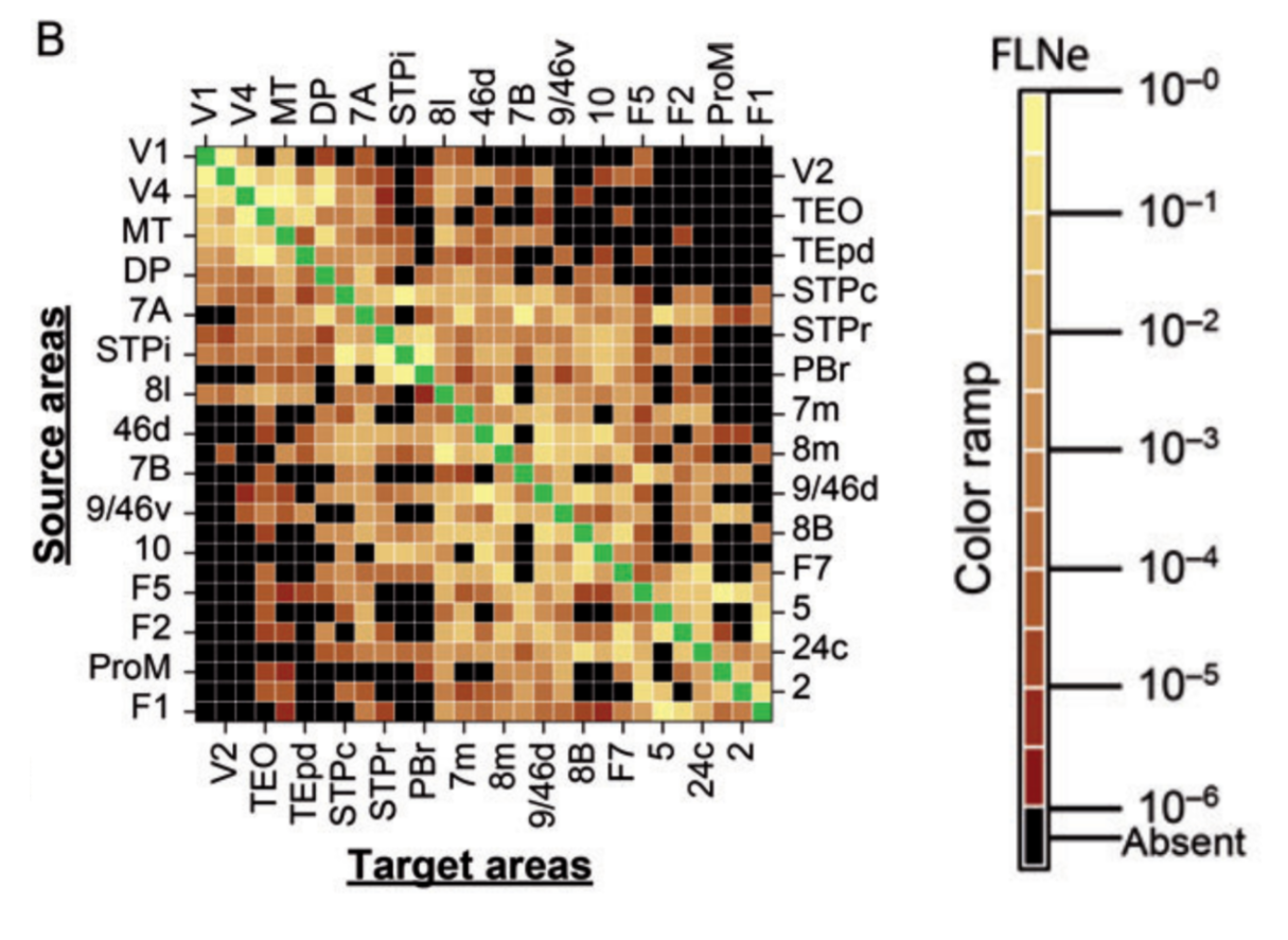
For rodents and primates, we must settle for statistical summaries and combine the data-driven bottom-up approach to understanding the brain with a computational-theory-driven top-down approach. The advances described by Wang et al. focus on the intermediate level 2. An important summary statistic at this level is the fraction of labeled neurons (FLN), which describes, for a retrograde tracer injected in a given region, in what proportions upstream regions contribute incoming axonal projections.
Matrix of directed connectivity strength among areas of the macaque cortex from Markov et al. (2014). Results are based on retrograde tracing from injections 29 cortical areas (those shown). Of all possible pairs of areas, about one third is reciprocally connected, about one third is unidirectionally connected, and about one third is unconnected. However, the strength of connectivity varies over five orders of magnitude.
Several insights emerged from tracer-based connectivity:
The strength of inter-area connectivity decays roughly exponentially with the areas’ distance in the brain.
Some pairs of areas are connected, but very sparsely. Other pairs of areas have a massive tract of fibers between them. Connectivity strengths vary by five orders of magnitudes.
The structural connectivity, in combination with a generic model of the excitatory/inhibitory local microcircuits, can be used as a basis for simulation of the network dynamics. The emergent dynamics is broadly consistent with neurophysiological observations, including slower, more integrative responses in regions further removed from the sensory input, which receive a larger proportion of their input through a broad distribution of paths through the network.
Laminar origins of connections differ between feedforward and feedback connections. Feedforward connection tend to originate in supragranular and feedback connections in infragranular layers. Modeling superficial and deep layers with separate excitatory/inhibitory microcircuits and using lamina-specific connectivity enables modeling of more detailed hierarchical dynamics, including the association of gamma with feedforward signals and alpha/beta with feedback.
A network model in which long-range excitation is tempered with local inhibition can explain threshold-dependent dynamics, where weak inputs fail to be propagated and inputs exceeding a threshold ignite a global response.
When a brain is scaled up , the number of possible pairwise connections grows as the square of the number of units to be connected (e.g. neurons or areas, depending on the level at which connectivity is considered). Full connectivity, thus, is much less costly in a small brain. This means that connectivity and component placement are less constrained in a small brain. Consistently with this simple fact, the macaque brain has connections among about two thirds of all pairs of areas (half of them reciprocal), whereas the mouse brain has 97% of all possible inter-area connections. The marmoset, a much smaller primate, may have somewhat more widely distributed connectivity than the macaque, but not to the extent predicted by its smaller-scale brain. Its connectivity is in fact quite similar to that of the macaque. Species and scaling both seem to matter to the overall degree of inter-area connectivity.
These models take a bottom-up approach in which the structural constraints provided by the tracer studies and descriptions of the cortical microcircuit are used to simulate global activity dynamics. Aspects of these dynamics, such as longer timescales in higher regions are suggestive of computational functions like evidence integration. However, the models do not perform task-related information processing, and so do not explain any cognitive functions. What is still missing is the integration of the bottom-up approach to modeling with the top-down approach of deep recurrent neural networks, where parameters are optimized for a model to perform a nontrivial perceptual, cognitive, or motor control task.
Suggestions for improvements in case the paper is revised
The paper is well-written and engaging. It’s great that it links structure to dynamics and points toward links between structure and computational function, which remain to be elaborated over the next decade. My main suggestion is to slightly expand this very concise piece with a view to (a) clarifying things that are currently a little too dense and (b) adding some elements that would make the paper even more useful to its readers.
Useful additions to consider include:
A table that compares the different available connectomic datasets in terms of the information provided and the information missing, and links to open-science resources to help neuroscientists use of the structural constraints for theory and modeling of function.
An update to the famous Felleman and van Essen (1991) diagram, with area sizes and directed, weighted connections. This seems very important for the field to have. Is it already available or can it be constructed with relative ease, at least for a subset of the regions, e.g. the macaque visual system?
A discussion of how the new connectomic data can be used to constrain brain-computational models (i.e. models that simulate the information processing enabling the brain to perform an ecologically relevant task such as visual recognition, categorization, navigation, or reaching).
Minor points
The correlation between inter-area connection-weight matrices from diffusion imaging and cellular tracers is cited as 0.59, and cellular tracing is referred to as ground truth. However, tracing also provides merely summary statistical information and is affected by sample error. Have the reliabilities of diffusion-based and cellular-tracing-based inter-area connection-weight estimates been established? It would be good to consider these in interpreting the consistency between the two techniques.
Second, the weight of connection (if present) between two areas decays exponentially with their distance (the exponential distance rule) [17].
Here it would be great to elaborate on the concept of distance. I assume what is meant is the Euclidean distance in the folded cortex. Readers may wonder if the cortical geodesic distance or the tract length in the white matter are more relevant. Some readers may even think of the hierarchical distance. Good to clarify and address these different notions of distance.
Open review of “Post-Publication Peer Review for Real” by Koki Ikeda, Yuki Yamada, and Kohske Takahashi (pp2020)
[I7R8]
Our system of pre-publication peer review is a relict of the age when the only way to disseminate scientific papers was through print media. Back then the peer evaluation of a new scientific paper had to precede its publication, because printing (on actual paper if you can believe it) and distributing the physical print copies is expensive. Only a small selection of papers could be made accessible to the entire community.
Now the web enables us to make any paper instantly accessible to the community at negligible cost. However, we’re still largely stuck with pre-publication peer review, despite its inherent limitations: to a small number of preselected reviewers who operate in isolation from and without the scrutiny of the community.
People familiar with the web who have considered, from first principles, how a scientific peer review system should be designed tend to agree that it’s better to make a new paper publicly available first, so the community can take note of the work and a broader set of opinions can contribute to the evaluation. Post-publication peer review also enables us to make the evaluation transparent: Peer reviews can be open responses to a new paper. Transparency promises to improve reviewers’ motivation to be objective, especially if they choose to sign and take responsibility for their reviews.
We’re still using the language of a bygone age, whose connotations make it hard to see the future clearly:
A paper today is no longer made of paper — but let’s stick with this one.
A preprint is not something that necessarily precedes the publication in print media. A better term would be “published paper”.
The term publication is often used to refer to a journal publication. However, preprints now constitute the primary publications. First, a preprint is published in the real sense: the sense of having been made publicly available. This is in contrast to a paper in Nature, say, which is locked behind a paywall, and thus not quite actually published. Second, the preprint is the primary publication in that it precedes the later appearance of the paper in a journal.
Scientists are now free to use the arXiv and other repositories (including bioRxiv and PsyArXiv) to publish papers instantly. In the near future, peer review could be an open and open-ended process. Of course papers could still be revised and might then need to be re-evaluated. Depending on the course of the peer evaluation process, a paper might become more visible within its field, and perhaps even to a broader community. One way this could happen is through its appearance in a journal.
The idea of post-publication peer review has been around for decades. Visions for open post-publication peer review have been published. Journals and conferences have experimented with variants of open and post-publication peer review. However, the idea has yet to revolutionize the scientific publication system.
In their new paper entitled “Post-publication Peer Review for Real”, Ikeda, Yamada, and Takahashi (pp2020) argue that the lack of progress with post-publication peer review reflects a lack of motivation among scientists to participate. They then present a proposal to incentivize post-publication peer review by making reviews citable publications published in a journal. Their proposal has the following features:
Any scientist can submit a peer review on any paper within the scope of the journal that publishes the peer reviews (the target paper could be published either as a preprint or in any journal).
Peer reviews undergo editorial oversight to ensure they conform to some basic requirements.
All reviews for a target paper are published together in an appealing and readable format.
Each review is a citable publication with a digital object identifier (DOI). This provides a new incentive to contribute as a peer reviewer.
The reviews are to be published as a new section of an existing “journal with high transparency”.
Ikeda at al.’s key point that peer reviews should be citable publications is solid. This is important both to provide an incentive to contribute and also to properly integrate peer reviews into the crystallized record of science. Making peer reviews citable publications would be a transformative and potentially revolutionary step.
The authors are inspired by the model of Behavioral and Brain Sciences (BBS), an important journal that publishes theoretical and integrative perspective and review papers as target articles, together with open peer commentary. The “open” commentary in BBS is very successful, in part because it is quite carefully curated by editors (at the cost of making it arguably less than entirely “open” by modern standards).
BBS was founded by Stevan Harnad, an early visionary and reformer of scientific publishing and peer review. Harnad remained editor-in-chief of BBS until 2002. He explored in his writings what he called “scholarly skywriting“, imagining a scientific publication system that combines elements of what is now known as open-notebook science and research blogging with preprints, novel forms of peer review, and post-publication peer commentary.
If I remember correctly, Harnad drew a bold line between peer review (a pre-publication activity intended to help authors improve and editors select papers) and peer commentary (a post-publication activity intended to evaluate the overall perspective or conclusion of a paper in the context of the literature).
I am with Ikeda et al. in believing that the lines between peer review and peer commentary ought to be blurred. Once we accept that peer review must be post-publication and part of a process of community evaluation of new papers, the prepublication stage of peer review falls away. A peer review, then, becomes a letter to both the community and to the authors and can serve any combination of a broader set of functions:
to explain the paper to a broader audience or to an audience in an adjacent field,
to critique the paper at the technical and conceptual level and possibly question its conclusions,
to relate it to the literature,
to discuss its implications,
to help the authors improve the paper in revision by adding experiments or analyses and improving the exposition of the argument in text and figures.
An example of this new form is the peer review you are reading now. I review only papers that have preprints and publish my peer reviews on this blog. This review is intended for both the authors and the community. The authors’ public posting of a preprint indicates that they are ready for a public response.
Admittedly, there is a tension between explaining the key points of the paper (which is essential for the community, but not for the authors) and giving specific feedback on particular aspects of the writing and figures (which can help the authors improve the paper, but may not be of interest to the broader community). However, it is easy to relegate detailed suggestions to the final section, which anyone looking only to understand the big picture can choose to skip.
Importantly, the reviewer’s judgment of the argument presented and how the paper relates to the literature is of central interest to both the authors and the community. Detailed technical criticism may not be of interest to every member of the community, but is critical to the evaluation of the claims of a paper. It should be public to provide transparency and will be scrutinized by some in the community if the paper gains high visibility.
A deeper point is that a peer review should speak to the community and to the authors in the same voice: in a constructive and critical voice that attempts to make sense of the argument and to understand its implications and limitations. There is something right, then, about merging peer review and peer commentary.
While reading Ikeda et al.’s review of the evidence that scientists lack motivation to engage in post-publication peer review, I asked myself what motivates me to do it. Open peer review enables me to:
more deeply engage the papers I review and connect them to my own ideas and to the literature,
more broadly explore the implications of the papers I review and start bigger conversations in the community about important topics I care about,
have more legitimate power (the power of a compelling argument publicly presented in response to the claims publicly presented in a published paper),
have less illegitimate power (the power of anonymous judgment in a secretive process that decides about publication of someone else’s work)
take responsiblity for my critical judgments by subjecting them to public scrutiny
make progress with my own process of scientific insight
help envision a new form of peer review that could prove positively transformative
In sum, open post-publication peer review, to me, is an inherently more meaningful activity than closed pre-publication peer review. I think there is plenty of motivation for open post-publication peer review, once people overcome their initial uneasiness about going transparent. A broader discussion of researcher motivations for contributing to open post-publication peer review is here.
That said, citability and DOIs are essential, and so are the collating and readability of the peer reviews of a target paper. I hope Ikeda et al. will pursue their idea of publishing open post-publication peer reviews in a journal. Gradually, and then suddenly, we’ll find our way toward a better system.
Suggestions for improvements
(1) The proposal raises some tricky questions that the authors might want to address:
Which existing “journal with high transparency” should this be implemented in?
Should it really be a section in an existing journal or a new journal (e.g. the “Journal of Peer Reviews in Psychology”)?
Are the peer reviews published immediately as they come in, or in bulk once there is a critical mass?
Are new reviews of a target paper to be added on an ongoing basis in perpetuity?
How are the target papers to be selected? Should their status as preprints or journal publications make any difference?
Why do we need to stick with the journal model? Couldn’t commentary sections on preprint servers solve the problem more efficiently — if they were reinvented to provide each review also as a separate PDF with beautiful and professional layout, along with figure and LaTeX support and, critically, citability and DOIs?
Consider addressing some of these questions to make the proposal more compelling. In particular, it seems attractive to find an efficient solution linked to preprint servers to cover large parts of the literature. Can the need for editorial work be minimized and the critical incentive provided through beautiful layout, citability, and DOIs?
(2) Cite and and discuss some of Stevan Harnad’s contributions. Some of the ideas in this edited collection of visions for post-publication peer review may also be relevant.
A recent large-scale survey reported that 98% of researchers who participated in the study agreed that the peer-review system was important (or extremely important) to ensure the quality and integrity of science. In addition, 78.8% answered that they were satisfied (or very satisfied) with the current review system (Publon, 2018) . It is probably true that peer-review has been playing a significant role to control the quality of academic papers (Armstrong, 1997) . The latter result, however, is rather perplexing, since it has been well known that sometimes articles could pass through the system without their flaws being revealed (Hopewell et al., 2014) , results could not be reproduced reliably (e.g. Open Science Collaboration, 2015) , decisions were said to be no better than a dice roll (Lindsey, 1988; Neff & Olden, 2006) , and inter-reviewer agreement was estimated to be very low (Bornmann et al., 2010).
(3) Consider disentangling the important pieces of evidence in the above passage a little more. “Perplexing” seems the wrong word here: Peer review can be simultaneously the best way to evaluate papers and imperfect. It would be good to separate mere evidence that mistakes happen (which appears unavoidable), from the stronger criticism that peer review is no better than random evaluations. A bit more detail on the cited results suggesting it is no better than random would be useful. Is this really a credible conclusion? Does it require qualifications?
The low reliability across reviewers is especially disturbing and raises serious concerns about the effectiveness of the system, because we now have empirical data showing that inter-rater agreement and precision could be very high, and they robustly predict the replicability of previous studies, when the information about others’ predictions are shared among predictors (Botvinik-Nezer et al., 2020; Camerer et al., 2016, 2018; Dreber et al., 2015; Forsell et al., 2019) . Thus, the secretiveness of the current system could be the unintended culprit of its suboptimality.
(4) Consider revising the above passage. Inter-reviewer agreement is an important metric to consider. However, even zero correlation between reviewer’s ratings does not imply that the reviews are random. Reviewers may focus on different criteria. For example, if one reviewer judged primarily the statistical justification of the claims and another primarily the quality of the writing, the correlation between their ratings could be zero. However, the average rating would be a useful indicator of quality. Averaging ratings in this context does not serve merely to reduce the noise in the evaluations, it also serves to compromise between different weightings of the criteria of quality.
Interaction among reviewers that enables them to adjust their judgments can fundamentally enhance the review process. However, inter-rater agreement is an ambiguous measure, when the ratings are not independent.
However, BBS commentary is different from them in terms of that it employs an “open” system so that anyone can submit the commentary proposal at will (although some commenters are arbitrarily chosen by the editor). This characteristic makes BBS commentary much more similar to PPPR than other traditional publications.
(5) Consider revising. Although BBS commentaries are nothing like traditional papers (typically much briefer statements of perspective on a target paper) and are a form of post-publication evaluation, they are also very distinct in form and content. I think Stevan Harnad made this point somewhere.
Next and most importantly, the majority of researchers find no problem with their incentives to submit an article as a BBS commentary, because they will be considered by many researchers and institutes to be equivalent to a genuine publication and can be listed on one’s CV. Therefore, researchers have strong incentives to actively publish their reviews on BBS .
(6) Consider revising. It’s a citable publication, yes. However, it’s in a minor category, nowhere near a primary research paper or a full review or perspective paper.
There seem to be at least two reasons for this uniqueness. Firstly, BBS is undoubtedly one of the most prestigious journals in psychology and its related areas, with a 17.194 impact factor for the year 2018. Secondly, the commentaries are selected by the editor before publication, so their quality is guaranteed at least to some extent. Critically, no current PPPR has the features comparable to these in BBS.
(7) Consider revising. While this is true for BBS, I don’t see how a journal of peer reviews that is open to all articles within a field, including preprints, as the target papers could replicate the prestige of BBS. This passage doesn’t seem to help the argument in favor of the new system as currently proposed. However, you might revise the proposal. For example, I could imagine a “Journal of Peer Commentary in Psychology” applying the BBS model to editorially selected papers of broad interest.
To summarize, we might be able to create a new and better PPPR system by simply combining the advantages of BBS commentary – (1) strong incentive for commenters and (2) high readability – with those of the current PPPRs – (3) unlimited target selection and (4) unlimited commentary accumulation -. In the next section, we propose a possible blueprint for the implementation of these ideas, especially with a focus on the first two, because the rest has already been realized in the current media.
(8) Consider revising. The first two points seem at a strong tension with the second two points. Strong incentive to review requires highly visible target publications, which isn’t possible if target selection is unlimited. High readability also appears compromised when reviews come in over a long period and there is no limit to their number. This should at least be discussed.
Among the features that seem critical to the successful implementation of PPPR, strong incentives for commenters is probably the most important factor. We speculated that BBS has achieved this goal by providing the commentaries a status equivalent to a standard academic paper. Furthermore, this is probably realized by the journal’s two unique characteristics: its academic prestige and the selection of commentaries by the editor. Based on these considerations, we propose the following plans for the new PPPR system.
(9) Consider revising. As discussed above, the commentaries do not quite have “equivalent” status to a standard academic paper.
Montobbio, Bonnasse-Gahot, Citti, & Sarti (pp2019) present an interesting model of lateral connectivity and its computational function in early visual areas. Lateral connections emanating from each unit drive other units to the degree that they are similar in their receptive profiles. Two units are symmetrically laterally connected if they respond to stimuli in the same region of the visual field with similar selectivity.
More precisely, lateral connectivity in this model implements a diffusion process in a space defined by the similarity of bottom-up filter templates. The similarity of the filters is measured by the inner product of the filter weights. Two filters that do not spatially overlap, thus, are not similar. Two filters are similar to the extent that their filters don’t merely overlap, but have correlated weight templates. Connecting units in proportion to their filter similarity results in a connectivity matrix that defines the paths of diffusion. The diffusion amounts to a multiplication with a convolution matrix. It is the activations (after the ReLU nonlinearity) that form the basis of the linear diffusion process.
The idea is that the lateral connections implement a diffusive spreading of activation among units with similar filters during perceptual inference. The intuitive motivation is that the spreading activation fills in missing information or regularizes the representation. This might make the representation of an image compromised by noise or distortion more like the representation of its uncompromised counterpart.
Instead of performing n iterations of the lateral diffusion at inference, we can equivalently take the convolutional matrix to the n-th power. The recurrent convolutional model is thus equivalent to a feedforward model with the diffusion matrix multiplication inserted after each layer.
Montobbio’s model for MNIST
In the context of Gabor-like orientation-selective filters,the proposed formula for connectivity results in an anisotropic kernel of lateral connectivity that looks plausible in that it connects approximately collinear edge filters. This is broadly consistent with anatomical studies showing that V1 neurons selective for oriented edges form long-range (>0.5 mm in tree shrew cortex) horizontal connections that preferentially target neurons selective for collinear oriented edges.
Figure from Bosking et al. (1997). Long-range lateral connections of oriented-edge-selective neurons in tree-shrew V1 preferentially project to other neurons selective for collinear oriented edges.
Since the similarity between filters is defined in terms of the bottom-up filter templates, it can be computed for arbitrary filters, e.g. filters learned through task training. The lateral connectivity kernel for each filter, thus, does not have to be learned through experience. Adding this type of recurrent lateral connectivity to a convolutional neural network (CNN), thus, does not increase the parameter count.
The authors argue that the proposed connectivity makes CNNs more robust to local perturbations of the image. They tested 2-layer CNNs on MNIST, Kuzushiji-MNIST, Fashion-MNIST, and CIFAR-10. They present evidence that the local anisotropic diffusion of activity improves robustness to noise, occlusions, and adversarial perturbations.
Overall, the authors took inspiration from visual psychophysics (Field et al. 1992; Geisler et al. 2001) and neurobiology (Bosking et al. 1997), abstracted a parsimonious mathematical model of lateral connectivity, and assessed the computational benefits of the model in the context of CNNs that perform visual recognition tasks. The proposed diffusive lateral activation might not be the whole story of lateral and recurrent connectivity in the brain, but it might be part of the story. The idea deserves careful consideration.
The paper is well written and engaging. I’m left with many questions as detailed below. In case the authors chose to revise the paper, it would be great to see some of the questions addressed, a deeper exploration of the functional mechanism underlying the benefits, and some more challenging tests of performance.
Figure from Geisler et al. (2001). Edge elements tend to be locally approximately collinear in natural images. Given that there is an orientated edge segment (shown as horizontal) in a particular location (shown in the center), the arrangement shows in what direction each orientation (oriented line) is most probable for each distance to the reference location.
Questions and thoughts
1 Can the increase in robustness be attributed to trivial forms of contextual integration?
If the filters were isotropic Gaussian blobs, then the diffusion process would simply blur the image. Blurring can help reduce noise and might reduce susceptibility to adversarial perturbations (especially if the adversary is not enabled to take this into account). Image blurring could be considered the layer-0 version of the proposed model. What is its effect on performance?
Consider another simplified scenario: If the network were linear, then the lateral connectivity would modify the effective filters, but each filter would still be a linear combination of the input. The model with lateral connectivity could thus be replaced by an equivalent feedforward model with larger kernels. Larger kernels might yield responses that are more robust to noise. Here the activation function is nonlinear, but the benefits might work similarly. It would be good to assess whether larger kernels in a feedforward network bring similar benefits to generalization performance.
2 Were the adversarial perturbations targeted at the tested model?
Robustness to adversarial attack should be tested using adversarial examples targeting each particular model with a given combination of numbers of iterations of lateral diffusion in layers 1 and 2. Was this the case?
3 Is the lateral diffusion process invertible?
The lateral diffusion is a linear transform that maps to a space of equal dimension (like Gaussian blurring of an image).
If the transform were invertible, then it would constitute the simplest possible change (linear, information preserving) to the representational geometry (as characterized by the Euclidean representational distance matrix for a set of stimuli). To better understand why this transform helps, then, it would be interesting to investigate how it changes the representational geometry for a suitable set of stimuli.
If lateral diffusion were not invertible, then it is perhaps best thought of as an intelligent type of pooling (despite the output dimension being equal to the input dimension).
4 Do the lateral connections make representations of corrupted images more similar to representations of uncorrupted versions of the same images?
The authors offer an intuitive explanation of the benefits to performance: Lateral diffusion restores the missing parts or repairs what has been corrupted (presumably using accurate prior information about the distribution of natural images). One could directly assess whether this is the case by assessing whether lateral diffusion moves the representation of a corrupted image closer to the representation of its uncorrupted variant.
5 Do correlated filter templates imply correlated filter responses under natural stimulation?
Learned filters reflect features that occur in the training images. If each image is composed of a mosaic of overlapping features, it is intuitive that filters whose templates overlap and are correlated will tend to co-occur and hence yield correlated responses across natural images. The authors seem to assume that this is true. But is there a way to prove that the correlations between filter templates really imply correlation of the filter outputs under natural stimulation? For independent noise images, filters with correlated templates will surely produce correlated outputs. However, it’s easy to imagine stimuli for which filters with correlated templates yield uncorrelated or anticorrelated outputs.
6 Does lateral connectivity reflecting the correlational structure of filter responses under natural stimulation work even better than the proposed approach?
Would the performance gains be larger or smaller if lateral connectivity were determined by filter-output correlation under natural stimulation, rather than by filter-template similarity?
Is filter-template similarity just a useful approximation to filter-output correlation under natural stimulation, or is there a more fundamental computational motivation for using it?
7 How does the proposed lateral connectivity compare to learned lateral connectivity when the number of connections (instead of the number of parameters) is matched?
It would be good to compare CNNs with lateral diffusive connectivity to recurrent convolutional neural networks (RCNNs) for matched sizes of bottom-up and lateral filters (and matched numbers of connections, not parameters). In addition, it would then be interesting to initialize the RCNNs with diffusive lateral connectivity according to the proposed model (after initial training without lateral connections). Lateral connections could precede (as in typical RCNNs) or follow (as in KerCNNs) the nonlinear activation function.
8 Does the proposed mechanism have a motivation in terms of a normative model of visual inference?
Can the intuition that lateral connections implement shrinkage to a prior about natural image statistics be more explicitly justified?
If the filters serve to infer features of a linear generative model of the image, then features with correlated templates are anti-correlated given the image (competing to explain the same variance). This suggests that inhibitory connections are needed to implement the dynamics for inference. Cortex does rely on local inhibition. How does local inhibitory connectivity fit into the picture?
Can associative filling in and competitive explaining away be reconciled and combined?
Strengths
A mathematical model of lateral connectivity, motivated by human visual contour integration and studies on V1 long-range lateral connectivity, is tested in terms of the computational benefits it brings in the context of CNNs that recognize images.
The model is intuitive, elegant, and parsimonious in that it does not require learning of additional parameters.
The paper presents initial evidence for improved generalization performance in the context of deep convolutional neural networks.
Weaknesses
The computational benefits of the proposed lateral connectivity is tested only in the context of toy tasks and two-layer neural networks.
Some trivial explanations for the performance benefits have not been ruled out yet.
It’s unclear how to choose the number of iterations of lateral diffusion for each of the the two layers, and choosing the best combination might positively bias the estimate of the gain in accuracy.
Figure from Boutin et al. (pp2019) showing how feedback from layer 2 to layer 1 in a sparse deep predictive coding model trained on natural images can give rise to collinear “association fields” (a concept suggested by Field et al. (1993) on the basis of psychophysical experiments). Montobbio et al. plausibly suggest that direct lateral connections may contribute to this function.
Figure from Montobbio et al. showing the kinds of perturbations that lateral connectivity rendered the networks more robust to.
Minor point
“associated to” -> “associated with” (in several places)
Nakai and Nishimoto (pp2019) had each of six subjects perform 103 naturalistic cognitive tasks during functional magnetic resonance imaging (fMRI) of their brain activity. This type of data could eventually enable us to more compellingly characterize the localization of cognitive task components across the human brain.
What is unique about this paper is the fact that it explores the space of cognitive tasks more systematically and comprehensively than any previous fMRI study I am aware of. It’s important to have data from many tasks in the same subjects to more quantitatively model how cognitive components, implemented in different parts of the brain, contribute in combination to different tasks.
The authors describe the space of tasks using a binary task-type model (with indicators for task components) and a continuous cognitive-factor model (with prior information from the literature incorporated via Neurosynth). They perform encoding and decoding analyses and investigate the clustering of task-related brain activity patterns. The model-based analyses are interesting, but also a bit hard to interpret, because they reveal the data only indirectly: through the lens of the models – and the models are very complex. It would be good to see some more basic “data-driven” analyses, as the title suggests.
However, the more important point is that this is a visionary contribution from an experimental point of view. The study pushes the envelope of cognitive fMRI. The biggest novel contributions are:
the task set (with its descriptive models)
the data (in six subjects)
Should the authors choose to continue to work on this, my main suggestions are (1) to add some more interpretable data-driven analyses, and (2) to strengthen the open science component of the study (by sharing the data, task and analysis code, and models), so that it can form a seed for much future work that builds on these tasks, expanding the models, the data, and the analyses beyond what can be achieved by a single lab.
This rich set of tasks and human fMRI responses deserves to be analyzed with a wider array of models and methods in future studies. For example, it would be great in the future to test a wide variety of task-descriptive models. Eventually it might also be possible to build neural network models that can perform the entire set of tasks. Explaining the measured brain-activity with such brain-computational models would get us closer to understanding the underlying information processing. In addition, the experiment deserves to be expanded to more subjects (perhaps 100). This could produce a canonical basis for revisiting human cognitive fMRI at a greater level of rigor. These directions may not be realistic for a single study or a single lab. However, this paper could be seminal to the pursuit of these directions as an open science endeavor across labs.
Improvements to consider if the authors chose to revise the paper
(1) Reconsider the phrase “data-driven models” (title)
The phrase “data-driven models” suggests that the analysis is both data-driven and model-based. This suggests the conceptualization of data-driven and model-based as two independent dimensions.
In this conceptualization, an analysis could be low on both dimensions, restricting the data to a small set (e.g. a single brain region) and failing to bring theory into the analysis through a model of some complexity (e.g. instead computing overall activation in the brain region for each experimental condition). Being high on both dimensions, then, appears desirable. It would mean that the assumptions (though perhaps strong) are explicit in the model (and ideally justified), and that the data still richly inform the results.
Arguably this is the case here. The models the authors used have many parameters and so the data richly inform the results. However, the models also strongly constrain the results (and indeed changing the model might substantially alter the results – more on that below).
But an alternative conceptualization, which seems to me more consistent with popular usage of these terms, is that there is a tradeoff between data-driven and model-based. In this conceptualization the overall richness of the results (how many independent quantities are reported) is considered a separate dimension. Any analysis combines data and assumptions (with the latter ideally made explicit in a model). If the model assumptions are weak (compared to the typical study in the same field), an analysis is referred to as data-driven. If the model assumptions are strong, then an analysis is referred to as model-driven. In this conceptualization, “data-driven model” is an oxymoron.
(2) Perform a data-driven (and model-independent) analysis of how tasks are related in terms of the brain regions they involve
“A sparse task-type encoding model revealed a hierarchical organization of cognitive tasks, their representation in cognitive space, and their mapping onto the cortex.” (abstract)
I am struggling to understand (1) what exact claims are made here, (2) how they are justified by the results, and (3) how they would constrain brain theory if true. The phrases “organization of cognitive tasks” and “representation in cognitive space” are vague.
The term hierarchical (together with the fact that a hierarchical cluster analysis was performed) suggests that (a) the activity patterns fall in clusters rather than spreading over a continuum and (b) the main clusters contain nested subclusters.
However, the analysis does not assess the degree to which the task-related brain activity patterns cluster. Instead a complex task-type model (whose details and influence on the results the reader cannot assess) is interposed. The model filters the data (for example preventing unmodeled task components from influencing the clustering). The outcome of clustering will also be affected by the prior over model weights.
A simpler, more data-driven, and interpretable analysis would be to estimate a brain activity pattern for each task and investigate the representational geometry of those patterns directly. It would be good to see the representational dissimilarity matrix and/or and visualization (MDS or t-SNE) of these patterns.
To formally address whether the patterns fall into clusters (and hierarchical clusters), it would be ideal to inferentially compare cluster (and hierarchical cluster) models to continuous models. For example, one could fit each model to a training set and assess whether the models’ predictive performance differs on an independent test set. (This is in contrast to hierarchical cluster analysis, which assumes a hierarchical cluster structure rather than inferring the presence of such a structure from the data.)
(3) Perform a simple pairwise task decoding analysis
It’s great that the decoding analysis generalizes to new tasks. But this requires model-based generalization. It would be useful, additionally, to use decoding to assess the discriminability of the task-related activity patterns in a less model-dependent way.
One could fit a linear discriminant for each pair of tasks and test on independent data from the same subject performing the same two tasks again. (If the accuracy were replaced by the linear discriminant t value or crossnobis estimator, then this could also form the basis for point (2) above.)
“A cognitive factor encoding model utilizing continuous intermediate features by using metadata-based inferences predicted brain activation patterns for more than 80 % of the cerebral cortex and decoded more than 95 % of tasks, even under novel task conditions.” (abstract)
The numbers 80% and 95% are not meaningful in the absence of additional information (more than 80% of the voxel responses predicted significantly above chance level, and more than 95% of the tasks were significantly distinct from at least some other tasks). You could either add the information needed to interpret these numbers to the abstract or remove the numbers from the abstract. (The abstract should be interpretable in isolation.)
New behavioral monitoring and neural-net modeling techniques are revolutionizing animal neuroscience. How can we use the new tools to understand how brains implement cognitive processes? Musall, Urai, Sussillo and Churchland (pp2019) argue that these tools enable a less reductive approach to experimentation, where the tasks are more complex and natural, and brain and behavior are more comprehensively measured and modeled. (The picture above is Figure 1 of the paper.)
There have recently been amazing advances in measurement, modeling, and manipulation of complex brain and behavioral dynamics in rodents and other animals. These advances point toward the ultimate goal of total experimental control, where the environment as well as the animal’s brain and behavior are comprehensively measured and where both environment and brain activity can be arbitrarily manipulated. The review paper by Musall et al. focuses on the role that monitoring and modeling complex behaviors can play in the context of modern neuroscientific animal experimentation. In particular, the authors consider the following elements:
Rich task environments: Rodents and other animals can be placed in virtual-reality experiments where they experience complex visual and other sensory stimuli. Researchers can richly and flexibly control the virtual environment, combining naturalistic and unnaturalistic elements to optimize the experiment for the question of interest.
Comprehensive measurement of behavior: The animal’s complex behavior can be captured in detail (e.g. running on a track ball and being videoed to measure running velocity and turns as well as subtle task-unrelated limb movements). The combination of video and novel neural-net-model-based computer vision, enables researchers to track the trajectories of multiple limbs simultaneously with great precision. Instead of focusing on binary choices and reaction times, some researchers now use comprehensive and detailed quantitative measurements of behavioral dynamics.
Data-driven modeling of behavioral dynamics: The richer quantitative measurements of behavioral dynamics enable the data-driven discovery of the dynamical components of behavior. These components can be continuous or categorical. An example of categorical components are behavioral motifs (categories of similar behavioral patterns). Such motifs used to be inferred subjectively by researchers observing the animals. Today they can be inferred more objectively, using probabilistic models and machine learning. These methods can learn the repertoire of motifs, and, given new data, infer the motifs and the parameters of each instantiation of a motif.
Cognitive models of task performance: Cognitive models of task performance provide the latent variables that the animal’s brain must represent to be able to perform the task. The latent variables connect stimuli to behavioral responses and enable us to take a normative, top-down perspective: What information processing should the animal perform to succeed at the task?
Comprehensive measurement of neural activity: Techniques for measuring neural activity, including multi-electrode recording devices (e.g. Neuropixels) and optical imaging techniques (e.g. Calcium imaging) have advanced to enable the simultaneous measurement of many thousands of neurons with cellular precision.
Modeling of neural dynamics: Neural-network models provide task-performing models of brain-information processing. These models abstract sufficiently from neurobiology to be efficiently simulated and trained, but are neurobiologically plausible in that they could be implemented with biological components. (One might say that these models leave out biological complexity at the cellular scale so as to be able to better capture the dynamic complexity at a larger scale, which might help us understand how the brain implements control of behavior.)
The paper provides a great concise introduction to these exciting developments and describes how the new techniques can be used in concert to help us understand how brains implement cognition. The authors focus on the role of monitoring and modeling behavior. They stress the need to capture uninstructed movements, i.e. movements that are not required for task performance, but nevertheless occur and often explain large amounts of variance in neural activity. They also emphasize the importance of behavioral variation across trials, brain states, and individuals. Detailed quantitative descriptions of behavioral dynamics enable researchers to model nuisance variation and also to understand the variation of performance across trials, which can reflect variation related to the brain state (e.g. arousal, fear), cognitive strategy (different algorithms for performing the task), and the individual studied (after all, every mouse is unique –– see figure above, which is Figure 1 in the paper).
Improvements to consider in case the paper is revised
The paper is well-written and useful already. In case the authors were to prepare a revision, they could consider improving it further by addressing some of the following points.
(1) Add a figure illustrating the envisaged style of experimentation and modeling.
It might be helpful for the reader to have another figure, illustrating how the different innovations fit together. Such a figure could be based on an existing study, or it could illustrate an ideal for future experimentation, amalgamating elements from different studies.
(2) Clarify what is meant by “understanding circuits” and the role of NNs as “tools” and “model organisms”.
The paper uses the term “circuit” in the title and throughout as the explanandum. The term “circuit” evokes a particular level of description: above the single neuron and below “systems”. The term is associated with small subsets of interacting neurons (sometimes identified neurons), whose dynamics can be understood in detail.
This is somewhat at a tension with the approach of neural-network modeling, where there isn’t necessarily a one-to-one mapping between units in the model and neurons in the brain. The neural-network modeling would appear to settle for a somewhat looser relationship between the model and the brain. There is a case to be made that this is necessary to enable us to engage higher-level cognitive processes.
The authors hint at their view of this issue by referring to the neural-network models as “artificial model organisms”. This suggests a feeling that these models are more like other biological species (e.g. the mouse “model”) than like data-analytical models. However, models are never identical to the phenomena they capture and the relationship between model and empirical phenomenon (i.e. what aspects of the data the model is supposed to predict) must be separately defined anyway. So why not consider the neural-network models more simply as models of brain information processing?
(3) Explain how the insights apply across animal species.
The basic argument of the paper in favor of comprehensive monitoring and modeling of behavior appears to hold equally for C. elegans, zebrafish, flies, rodents, tree shrews, marmosets, macaques, and humans. However, the paper appears to focus on rodents. Does the rationale change across species? If so how and why? Should human researchers not consider the same comprehensive measurement of behavior for the very same reasons?
(4) Clarify the relation to similar recent arguments.
Several authors have recently argued that behavioral modeling must play a key role if we are to understand how the brain implements cognitive processes (Krakauer et al. 2017, Neuron [cited already]; Yamins & DiCarlo 2016, Nature Neuroscience; Kriegeskorte & Douglas 2018, Nature Neuroscience 2018). It would be interesting to hear how the authors see the relationship between these arguments and the one they are making.