[I7R8]
Rajesh Rao (pp2019) gives a concise review of the current state of the art in bidirectional brain-computer interfaces (BCIs) and offers an inspiring glimpse of a vision for future BCIs, conceptualized as neural co-processors.
A BCI, as the name suggests, connects a computer to a brain, either by reading out brain signals or by writing in brain signals. BCIs that both read from and write to the nervous system are called bidirectional BCIs. The reading may employ recordings from electrodes implanted in the brain or located on the scalp, and the writing must rely on some form of stimulation (e.g., again, through electrodes).
An organism in interaction with its environment forms a massively parallel perception-to-action cycle. The causal routes through the nervous system range in complexity from reflexes to higher cognition and memories at the temporal scale of the life span. The causal routes through the world, similarly, range from direct effects of our movements feeding back into our senses, to distal effects of our actions years down the line.
Any BCI must insert itself somewhere in this cycle – to supplement, or complement, some function. Typically a BCI, just like a brain, will take some input and produce some output. The input can come from the organism’s nervous system or body, or from the environment. The output, likewise, can go into the organism’s nervous system or body, or into the environment.
This immediately suggests a range of medical applications (Figs. 1, 2):
- replacing lost perceptual function: The BCI’s input comes from the world (e.g. visual or auditory signals) and the output goes to the nervous system.
- replacing lost motor function: The BCI’s input comes from the nervous system (e.g. recordings of motor cortical activity) and the output is a prosthetic device that can manipulate the world (Fig. 1).
- bridging lost connectivity or replacing lost nervous processing: The BCI’s input comes from the nervous system and the output is fed back into the nervous system (Fig. 2).
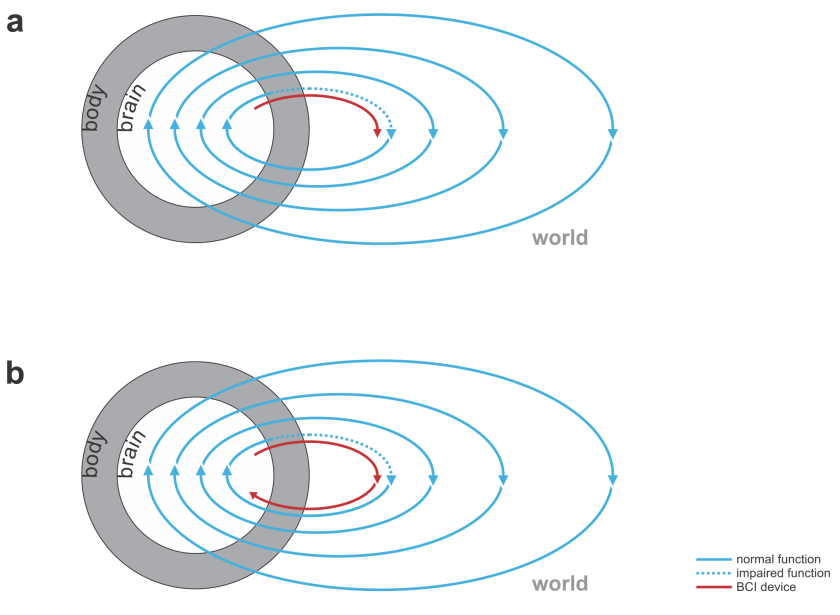 Fig. 1 | Uni- and bidirectional prosthetic-control BCIs. (a) A unidirectional BCI (red) for control of a prosthetic hand that reads out neural signals from motor cortex. The patient controls the hand using visual feedback (blue arrow). (b) A bidirectional BCI (red) for control of a prosthetic hand that reads out neural signals from motor cortex and feeds back tactile sensory signals acquired through artificial sensors to somatosensory cortex.
Beyond restoring lost function, BCIs have inspired visions of brain augmentation that would enable us to transcend normal function. For example, BCI’s might enable us to perceive, communicate, or act at higher bandwidth. While interesting to consider, current BCIs are far from achieving the bandwidth (bits per second) of our evolved input and output interfaces, such as our eyes and ears, our arms and legs. It’s fun to think that we might write a text in an instant with a BCI. However, what limits me in writing this open review is not my hands or the keyboard (I could use dictation instead), but the speed of my thoughts. My typing may be slower than the flight of my thoughts, but my thoughts are too slow to generate an acceptable text at the pace I can comfortably type.
But what if we could augment thought itself with a BCI? This would require the BCI to listen in to our brain activity as well as help shape and direct our thoughts. In other words, the BCI would have to be bidirectional and act as a neural co-processor (Fig. 3). The idea of such a system helping me think is science fiction for the moment, but bidirectional BCIs are a reality.
I might consider my laptop a very functional co-processor for my brain. However, it doesn’t include a BCI, because it neither reads from nor writes to my nervous system directly. It instead senses my keystrokes and sends out patterns of light, co-opting my evolved biological mechanisms for interfacing with the world: my hands and eyes, which provide a bandwidth of communication that is out of reach of current BCIs.
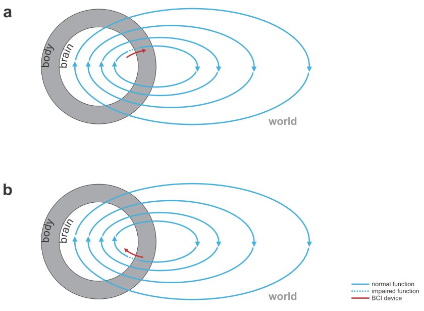
Fig. 2 | Bidirectional motor and sensory BCIs. (a) A bidirectional motor BCI (red) that bridges a spinal cord injury, reading signals from motor cortex and writing into efferent nerves beyond the point of injury or directly contacting the muscles. (b) A bidirectional sensory BCI that bridges a lesion along the sensory signalling pathway.
Rao reviews the exciting range of proof-of-principle demonstrations of bidirectional BCIs in the literature:
- Closed-loop prosthetic control: A bidirectional BCI may read out motor cortex to control a prosthetic arm that has sensors whose signals are written back into somatosensory cortex, replacing proprioceptive signals. (Note that even a unidirectional BCI that only records activity to steer the prosthetic device will be operated in a closed loop when the patient controls it while visually observing its movement. However, a bidirectional BCI can simultaneously supplement both the output and the input, promising additional benefits.)
- Reanimating paralyzed limbs: A bidirectional BCI may bridge a spinal cord injury, e.g. reading from motor cortex and writing to the efferent nerves beyond the point of injury in the spinal cord or directly to the muscles.
- Restoring motor and cognitive functions: A bidirectional BCI might detect a particular brain state and then trigger stimulation is a particular region. For example, a BCI may detect the impending onset of an epileptic seizure in a human and then stimulate the focus region to prevent the seizure.
- Augmenting normal brain function: A study in monkeys demonstrated that performance on a delayed-matching-to-sample task can be enhanced by reading out the CA3 representation and writing to the CA1 representation in the hippocampus (after training a machine learning model on the patterns during normal task performance). BCIs reading from and writing to brains have also been used as (currently still very inefficient) brain-to-brain communication devices among rats and humans.
- Inducing plasticity and rewiring the brain: It has been demonstrated that sequential stimulation of two neural sites A and B can induce Hebbian plasticity such that the connections from A to B are strengthened. This might eventually be useful for restoration of lost connectivity.
Most BCIs use linear decoders to read out neural activity. The latent variables to be decoded might be the positions and velocities capturing the state of a prosthetic hand, for example. The neural measurements are noisy and incomplete, so it is desirable to combine the evidence over time. The system should use not only the current neural activity pattern to decode the latent variables, but also the recent history. Moreover, it should use any prior knowledge we might have about the dynamics of the latent variables. For example, the components of a prosthetic arm are inert masses. Forces upon them cause acceleration, i.e. a change of velocity, which in turn changes the positions. The physics, thus, entails smooth positional trajectories.
When the neuronal activity patterns linearly encode the latent variables, the dynamics of the latent variables is also linear, and the noise is Gaussian, then the optimal way of inferring the latent variables is called a Kalman filter. The state vector for the Kalman filter may contain the kinematic quantities whose brain representation is to be estimated (e.g. the position, velocity, and acceleration of a prosthetic hand). A dynamics model that respects the laws of physics can help constrain the inference so as to obtain more reliable estimates of the latent variables.
For a perceptual BCI, similarly, the signals from the artificial sensors might be noisy and we might have prior knowledge about the latent variables to be encoded. Encoders, as well as decoders, thus, can benefit from using models that capture relevant information about the recent input history in their internal state and use optimal inference algorithms that exploit prior knowledge about the latent dynamics. Bidirectional BCIs, as we have seen, combine neural decoders and encoders. They form the basis for a more general concept that Rao introduces: the concept of a neural co-processor.
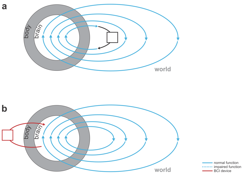
Fig. 3 | Devices augmenting our thoughts. (a) A laptop computer (black) that interfaces with our brains through our hands and eyes (not a BCI). (b) A neural co-processor that reads out neural signals from one region of the brain and writes in signals into another region of the brain (bidirectional BCI).
The term neural co-processor shifts the focus from the interface (where brain activity is read out and/or written in) to the augmentation of information processing that the device provides. The concept further emphasizes that the device processes information along with the brain, with the goal to supplement or complement what the brain does.
The framework for neural co-processors that Rao outlines generalizes bidirectional BCI technology in several respects:
- The device and the user’s brain jointly optimize a behavioral cost function:
BCIs from the earliest days have involved animals or humans learning to control some aspect of brain activity (e.g. the activity of a single neuron). Conversely, BCIs standardly employ machine learning to pick up on the patterns of brain activity that carry a particular meaning. The machine learning of patterns associated, say, with particular actions or movements is often followed by the patient learning to operate the BCI. In this sense mutual co-adaptation is already standard practice. However, the machine learning is usually limited to an initial phase. We might expect continual mutual co-adaptation (as observed in human interaction and other complex forms of communication between animals and even machines) to be ultimately required for optimal performance. - Decoding and encoding models are integrated: The decoder (which processes the neural data the device reads as its input) and encoder (which prepares the output for writing into the brain) are implemented in a single integrated model.
- Recurrent neural network models replace Kalman filters: While a Kalman filter is optimal for linear systems with Gaussian noise, recurrent neural networks provide a general modeling framework for nonlinear decoding and encoding, and nonlinear dynamics.
- Stochastic gradient descent is used to adjust the co-processor so as to optimize behavioral accuracy: In order to train a deep neural network model as a neural co-processor, we would like to be able to apply stochastic gradient descent. This poses two challenges: (1) We need a behavioral error signal that measures how far off the mark the combined brain-co-processor system is during behavior. (2) We need to be able to backpropagate the error derivatives. This requires that we have a mathematically specified model not only for the co-processor, but also for any further processing performed by the brain to produce the behavior whose error is to drive the learning. The brain-information processing from co-processor output to behavioral response is modeled by an emulator model. This enables us to backpropagate the error derivatives from the behavioral error measurements to the co-processor and through the co-processor. Although backpropagation proceeds through the emulator first, only the co-processor learns (as the emulator is not involved in the interaction and only serves to enable backpropagation). The emulator needs to be trained to emulate the part of the perception-to-action cycle it is meant to capture as well as possible.
The idea of neural co-processors provides an attractive unifying framework for developing devices that augment brain function in some way, based on artificial neural networks and deep learning.
Intriguingly, Rao argues that neural co-processors might also be able to restore or extend the brain’s own processing capabilities. As mentioned above, it has been demonstrated that Hebbian plasticity can be induced via stimulation. A neural co-processor might initially complement processing by performing some representational transformation for the brain. The brain might then gradually learn to predict the stimulation patterns contributed by the co-processor. The co-processor would scaffold the processing until the brain has acquired and can take over the representational transformation by itself. Whether this would actually work remains to be seen.
The framework of neural co-processors might also be relevant for basic science, where the goal is to build models of normal brain-information processing. In a basic-science context, the goal is to drive the model parameters to best predict brain activity and behavior. The error derivatives of the brain or behavioral predictions might be continuously backpropagated through a model during interactive behavior, so as to optimize the model.
Overall, this paper gives an exciting concise view of the state of the literature on bidirectional BCIs, and the concept of neural co-processors provides an inspiring way to think about the bigger picture and future directions for this technology.
Strengths
- The paper is well-written and gives a brief, but precise overview of the current state of the art in bidirectional BCI technology.
- The paper offers an inspiring unifying framework for understanding bidirectional BCIs as neural co-processors that suggests exciting future developments.
Weaknesses
- The neural co-processor idea is not explained as intuitively and comprehensively as it could be.
- The paper could give readers from other fields a better sense of quantitative benchmarks for BCIs.
Improvements to consider in revision
The text is already at a high level of quality. These are just ideas for further improvements or future extensions.
- The figure about neural co-processors could be improved. In particular, the author could consider whether it might help to
- clarify the direction of information flow in the brain and the two neural networks (clearly discernible arrows everywhere)
- illustrate the parallelism between the preserved healthy output information flow (e.g. M1->spinal cord->muscle->hand movement) and the emulator network
- illustrate the function intuitively using plausible choices of brain regions to read from (PFC? PPC?) and write to (M1? – flipping the brain?)
- illustrate an intuitive example, e.g. a lesion in the brain, with function supplemented by the neural co-processor
- add an external actuator to illustrate that the co-processor might directly interact with the world via motors as well as sensors
- clarify the source of the error signal
- The text on neural co-processors is very clear, but could be expanded by considering another example application in an additional paragraph to better illustrate the points made conceptually about the merits and generality of the approach.
- The expected challenges on the path to making neural co-processors work could be discussed in more detail.
- It would be good to clarify how the behavioral error signals to be backpropagated would be obtained in practice, for example, in the context of motor control.
- Should we expect that it might be tractable to learn the emulator and co-processor models under realistic conditions? If so, what applied and basic science scenarios might be most promising to try first?
- If the neural co-processor approach were applied to closed-loop prosthetic arm control, there would have to be two separate co-processors (motor cortex -> artificial actuators, artificial sensors -> sensory cortex) and so the emulator would need to model the brain dynamics intervening between perception and action.
- It would be great to include some quantitative benchmarks (in case they exist) on the performance of current state-of-the-art BCIs (e.g. bit rate) and a bit of text that realistically assesses where we are on the continuum between proof of concept and widely useful application for some key applications. For example, I’m left wondering: What’s the current maximum bit rate of BCI motor control? How does this compare to natural motor control signals, such as eye blinks? Does a bidirectional BCI with sensory feedback improve the bit rate (despite the fact that there is already also visual feedback)?
- It would be helpful to include a table of the most notable BCIs built so far, comparing them in terms of inputs, outputs, notable achievements and limitations, bit rate, and encoding and decoding models employed.
- The current draft lacks a conclusion that draws the elements together into an overall view.