Using performance-driven deep learning models to understand sensory cortex

In a new perspective piece in Nature Neuroscience, Yamins & Dicarlo (2016) discuss the emerging methodology and initial results in the literature of using deep neural nets with millions of parameters optimised for task performance to explain representations in sensory cortical areas. These are important developments. The authors explain the approach very well, also covering the historical progression toward it and its future potential.  Here are the key features of the approach as outlined by the authors.

(1) Complex models with multiple stages of nonlinear transformation from stimulus to response are used to explain high-level brain representations. The models are “stimulus computable” in the sense of fully specifying the computations from a physical description of the stimulus to the brain responses (avoiding the use of labels or judgments provided by humans).

(2) The models are neurobiologically plausible and “mappable”, in the sense that their components are thought to be implemented in specific locations in the brain. However, the models abstract from many biological details (e.g. spiking, in the reviewed studies).

(3) The parameters defining a model are specified by optimising the model’s performance at a task (e.g. object recognition). This is essential because deep models have millions of parameters, orders of magnitude too many to be constrained by the amounts of brain-activity data that can be acquired in a typical current study.

(4) Brain-activity data may additionally be used to define affine transformations of the model representations, so as to (a) fine-tune the model to explain the brain representations and/or (b) define the relationship between model units and measured brain responses in a particular individual.

(5) The resulting model is tested by evaluating the accuracy with which it predicts the representation of a set of stimuli not used in fitting the model. Prediction accuracy can be assessed at different levels of description:

  1. as the accuracy of prediction of a stimulus-response matrix,
  2. as the accuracy of prediction of a representational dissimilarity matrix, or
  3. as the accuracy of prediction of task-information decodability (i.e. are the decoding accuracies for a set of stimulus dichotomies correlated between model and neural population?).

A key insight is that the neural-predictive success of the models derives from combining constraints on architecture and function.

  • Architecture: Neuroanatomical and neurophysiological findings suggest (a) that units should minimally be able to compute linear combinations followed by static nonlinearities and (b) that their network architecture should be deep with rich multivariate representations at each stage. 
  • Function: Biological recognition performance and informal characterisations of high-level neuronal response properties suggest that the network should perform a transformation that retains high-level sensory information, but also emphasises behaviourally relevant categories and semantic dimensions. Large sets of labelled stimuli provide a constraint on the function to be computed in the form of a lookup table.

Bringing these constraints together has turned out to enable the identification of models that predict neural responses throughout the visual hierarchies better than any other currently available models. The models, thus, generalise not just to novel stimuli (Yamins et al. 2014; Khaligh-Razavi & Kriegeskorte 2014; Cadieu et al. 2014), but also from the constraints imposed on the mapping (e.g. mapping images to high-level categories) to intermediate-level representational stages (Güçlü & van Gerven 2015; Seibert et al. PP2016). Similar results are beginning to emerge for auditory representations.

The paper contains a useful future outlook, which is organised into sections considering improvements to each of the three components of the approach:

  • model architecture: How deep, what filter sizes, what nonlinearities? What pooling and local normalisation operations?
  • goal definition: What task performance is optimised to determine the parameters?
  • learning algorithm: Can learning algorithms more biologically plausible than backpropagation and potentially combining unsupervised and supervised learning be used?

In exploring alternative architectures, goals, and learning algorithms, we need to be guided by the known neurobiology and by the computational goals of the system (ultimately the organism’s survival and reproduction). The recent progress with neural networks in engineering provides the toolbox for combining neurobiologically plausible components and setting their parameters in a way that supports task performance. Alternative architectures, goals, and learning algorithms will be judged by their ability to predict neural representations of novel stimuli and biological behaviour.

The final section reflects on the fact that the feedfoward deep convolutional models currently very successful in this area only explain the feedforward component of sensory processing. Recurrent neural net models, which are also rapidly conquering increasingly complex tasks in engineering applications, promise to address these limitations of the initial studies using deep nets to explain sensory brain representations.

This perspective paper will be of interest to a broad audience of neuroscientists not themselves working with complex computational models, who are looking for a big-picture motivation of the approach and review of the most important findings. It will also be of interest to practitioners of this new approach, who will value the historical review and the careful motivation of each of the components of the methodology.


Deep net representational geometries become more similar to the ventral stream as performance is optimised


[R6I7]


Seibert, Yamins, Ardila, Hong, DiCarlo, and Gardner compared a deep convolutional neural network for visual object recognition to human ventral-stream representations as measured with fMRI (PP). The network was similar to the one described in Krizhevsky et al. (2012), the network that won the ImageNet competition that year with a large increase in performance compared to previous computer vision systems. The representations in the layers of the Krizhevsky deep net and similar models have been compared to human and monkey brain representations at different stages of the ventral stream previously (Yamins et al. 2013, Yamins et al. 2014; Khaligh-Razavi & Kriegeskorte 2014; Cadieu et al. 2014; Güçlü & van Gerven 2015). The present study is consistent with the previous results, generalises this line work to an interesting new set of test images, and investigates how the representational similarity of the model layers to the brain areas evolves as model performance is optimised. Results suggest that the optimisation of recognition performance increases representational similarity to visual areas, even for early and mid-level visual areas.

Model architecture: The convolutional network was inspired by that of Krizhevsky et al. (2012), using similar convolutional filter sizes, rectified linear units, the same pooling and local normalisation procedures, and data from ImageNet for training on 1000-class categorisation. However, the input images were downsampled to a substantially smaller size (120 x 120 pixels, instead of 224 x 224 pixels). Another major modification was that two intermediate fully connected layers (which contain most of the parameters in Krizhevsky et al.’s net) were omitted. This is reported to have no significant effect on recognition performance on an independent ImageNet test set.

Training and test stimuli: Like Krizhevsky et al., Seibert et al. trained the network by backpropagation to classify objects into 1000 categories. They used the very large ImageNet set of labelled images for model training and then presented the network and two human subjects with a different set of more controlled images: 1,785 grayscale images of 3D renderings of objects in many positions and views, superimposed to random natural backgrounds.

Representational similarity analysis: The authors compared the representational dissimilarity matrices (RDMs) between model layers and brain areas. They first randomly selected 1000 model features from a given layer, then reweighted these features, stretching and squeezing the representational space along its original axes, so as to maximise the RDM correlation between the model layer and the brain region. The maximisation of the RDM correlation was performed on the basis of 15 of the images for each of the 64 objects (different positions, views, and backgrounds). Using the fitted weights, they then re-estimated the model RDMs on the basis of the other 12 position-view combinations for the same 64 objects and computed the RDM correlation (Spearman) between model layer and brain region.


ScreenShot741

Detail of Figure 1 from the paper: Grayscale stimulus images were created by superimposing 3D models to natural backgrounds. The set strikes an interesting balance between naturalness and control. There were 8 objects from each of 8 categories (animals, boats, cars, chairs, faces, fruits, planes, tables) and each object was presented in 27 or 28 different combinations of position (including entirely nonoverlapping positions), view, and natural background image. For each of the 8 x 8 = 64 objects, they averaged response patterns to all the images that contained it, so as to compute 64 x 64-entry representational dissimilarity matrices (RDMs) using 1-Pearson correlation as the distance measure.


Related previous work: This work is closely related to recent papers by Yamins et al. (2013; 2014), Khaligh-Razavi et al. (2014), Cadieu et al. (2014), and Güçlü & van Gerven (2015). Yamins et al. showed that performance-optimised convolutional network models explain primate-IT neuronal recordings, with models performing better at object recognition also better explaining IT. Khaligh-Razavi et al. compared 37 computational model representations, including the layers of the Krizhevsky et al. (2012) model and a range of popular computer vision features, to human fMRI and monkey recording data (Kiani et al. 2007) and found that only the deep convolutional net, which was extensively trained to emphasize categorical divisions, could fully explain the IT data. They also showed that early visual cortex is well accounted for by earlier layers of the deep convolutional network (and by Gabor representations and other computer vision features). Cadieu et al. (2014) showed that among 6 different models, only Krizhevsky et al. (2012) and an even more powerful deep convolutional network by Zeiler & Fergus (2013) separate the categories in the representational space to a degree comparable to IT cortex. Güçlü & van Gerven (2015) investigated to what extent each layer of the model could explain the representations in each visual area of the ventral stream, finding rough correspondences between lower, intermediate, and higher model representations and early, mid-level, and higher ventral-stream regions, respectively.


How does the present work go beyond previous studies? The most striking novel contribution of this study is the characterisation of how representational similarity to visual areas develops as the neural net’s performance is optimised from a random initialisation. Unlike Yamins et al. (2014) and Cadieu et al. (2014), this study compares a convolutional network to the human ventral stream and, unlike Khaligh-Razavi & Kriegeskorte (2014), each image was presented in many positions and views and with many different backgrounds. The data is from only two subjects, but each subject underwent 9 sessions, so the total data set is substantial. The human fMRI data set is exciting in that it systematically varies category, exemplar, and accidental properties (position, view, background). However, the authors averaged across different images of each of the objects. I wonder if this data set has further potential for future analyses that don’t average across responses to different images.

Comparing many model representations to each of the areas of the visual system is a challenge requiring multiple studies. It’s great to see another study comparing the layers (including pooling layers and intermediate convolutional stages) alongside several control models (V1-like, V2-like, HMAX), which hadn’t been compared to deep convolutional networks before.


ScreenShot756

Figure 2 from the paper: Successive stages of the human ventral stream (V1, V2, V4, LOC) are best explained by successive layers of a deep convolutional neural net model. The representational geometry in V1 most resembles that of a lower and an intermediate layer of the network. The representational geometry in V2 most resembles that of an intermediate layer. And the representational geometries of V4 and LOC most resemble that of a higher layer of the network. Categories are reflected in clusters of response patterns in V4 and even more strongly in LOC. The same holds for higher layers of the network model.


Strengths

  • Model predictions of brain representational geometries are analysed as a function of model performance. This nicely demonstrates that it is not just the architecture, but performance optimisation that drives successful predictions of representations across all levels of the ventral stream.
  • Adds to the evidence that deep convolutional neural networks can explain the feedforward component of the stagewise representational transformations in the ventral visual stream.
  • Rich stimulus set of 1785 images that strikes an interesting balance between naturalism and control, independently varying objects and accidental properties.
  • Multiple data sets in each subject. This fMRI data set could in the future support tests of a wide variety of models.


Weaknesses

  • Statistical procedures are not clearly described and not fully justified. What type of generalisation does the crossvalidation scheme test for? What is being bootstrapped? Why are normal and independence assumptions relied on for inference, when bootstrapping the objects would enable straightforward tests that don’t require these assumptions?
  • The analysis is based on average response patterns across many different images for each object. This renders results more difficult to interpret.
  • Only two subjects.

Overall, this is a very nice study and a substantial contribution to the literature. However, the averaging across responses elicited by different images complicates the interpretation of the results and the statistical analyses need to be improved, better described, and fully justified – as detailed below. Although the overall results described in this review appear likely to hold up, I am not confident that the inferential results for particular model comparisons are reliable. (If concerns detailed below were substantively addressed, I would consider adjusting the reliability rating.)


Issues to consider addressing in a revision

(1) Can averaged response patterns elicited by different individual images be interpreted?

If we knew a priori that a region represents the objects with perfect invariance to position, view and background, then averaging across many images of the same objects that differ in these variables would make sense. However, we know that none of the regions is really invariant to position, view, and background, and gradually achieving some tolerance is one of the central computational challenges. The averaging will have differential effects in different regions as tolerance increases along the ventral stream. I don’t understand how to interpret the RDM for V1 given that it is based on averaged patterns. The object positions and backgrounds vary widely. Presumably different images of the same object are represented totally differently in V1. The averages should then form a tighter cluster of patterns (by factor 4 after averaging 16 images). Isn’t it puzzling then that the resulting RDM is still significantly correlated with the model? To explain this, do we have to assume that V1 actually represents the objects somewhat tolerantly (perhaps through feedback)? In a high-level representation tolerant to variation of accidental properties and sensitive to categorical differences, we expect the representations of the different images for a given object to be much more similar, so the averaging would have a smaller effect. All this confusion could be avoided by analysing patterns evoked by individual images. In addition, the emergence of tolerance across stages of processing could then be characterised.


(2) What type of generalisation does the crossvalidation scheme support?

Ideally, the crossvalidation should estimate the generalisation performance of the RDM prediction from the model for new images showing different objects. This is not the case here.

  • First, it appears that the brain data used for training (model weight fitting) and test (estimation of RDM correlation) are responses to the same set of images (all images). The weighting of the model features is estimated using a subset of 15 of the images for each object, and the RDM correlation between model and brain data assessed using 12 different images (different poses and backgrounds) of the same objects. This would seem to fall short of a test of generalisation to new images (even of the same objects) because all images are used (on the side of the brain responses) in the training procedure. Please clarify this issue.
  • Second, even if there was no overlap in the images used in training and test (on the side of either the model fitting or the brain data), the models are overfitted to the object set. Ideally, nonoverlapping sets of images of different objects should be used for training and testing. How about using a random subset of 4 of the objects in each category (32 in total) for fitting the weights and the other 32 objects for estimating the RDM correlation?

Overall, it seems unclear what type of generalisation these analyses test for. Let’s consider the issue of overfitting to the object set more closely. Currently, the weights w are fitted to 15 of the 27 images for a given object. In an idealised high-level representation invariant to the accidental variation, the two image sets will be identically represented. We expect the object representations to be in general position (no two on a point, no three on a line, no four on a plane and so on). Even if the 64 object representations were not at all clustered by category, but instead distributed randomly, we could linearly read out any categorical distinction and the decoder would generalise to the other 12 images. This is just to illustrate the expected effect of overfitting to the object set. In the present study, weights were fitted to predict RDMs not to discriminate categories. Fitting the 1000 scaling parameters to explain an RDM with 64*(64-1)/2 = about 2K dissimilarities should enable us to fit any RDM quite precisely. I would not be surprised if a noncategorical representation could fit a clearly categorical representation (block-diagonal RDM) in this context. The test-set correlations would then really just be a measure of the replicability of the brain RDMs – rather than a measure of the fit of the model. Regularisation might help ensure that different models are still distinguishable, but it also further complicates interpretation (see below).

Since higher regions are more tolerant, the training and test images are more similarly represented in these regions, and so we would expect greater positive overfitting bias on the estimated RDM correlation for higher regions regardless of the model. It is reassuring that the models still perform differently in LOC. However, the overfitting to the object set complicates interpretation.

The category decoding performance measure is similarly compromised by averaging across different images. Decoding performance as well (if I understood correctly) was tested by averaging different images for each object and training and testing on the same set of objects with different particular images in the test set. So the test is not a test of generalisation to different objects but to different images of the same objects. Again any representation uniquely representing each object (and having at least as many dimensions as the number of objects in both classes combined minus one, which is the case here) will appear to support linear category decoding, even if the distributions in representational space corresponding to the two categories (including the entire populations of objects they comprise) were not at all linearly separable and across-object generalisation performance were at chance level.


(3) Clarify the bootstrapping procedure used in model comparison

The first 6 times the term bootstrap is used, it is entirely unclear what entities are being resampled with replacement. The sampling of 1000 model units is explained in this context, and suggests that this is the resampling with replacement referred to as bootstrapping. Only on page 15 it says: “Our approach bootstraps over independent stimulus samples”. I’m not sure what multiple independent stimulus samples are meant here. Are the objects (averaged across images) resampled? Or are the images resampled? (The latter would necessitate re-estimating the object-average voxel responses to each object for each bootstrap sample.)


(4) Clarify and justify the test used for model comparison

The methods section states:

“Using the bootstrapping above, we computed p-values testing if Layer A better explained visual area X’s RDM than Layer B”

This suggests that a bootstrap test was used to compare models with respect to their RDM prediction performance. But then the model comparison test is described as follows:

“We use Fisher’s r-to-z transformation using Steiger (1980)’s approach to compute p-values for difference in correlation values (Lee and Preacher, 2013). The approach tests for equality of two correlation values from the same sample where one variable is held in common between the two coefficients (in our case, an RDM of a given visual area).”

The Steiger (1980) method for comparing two dependent correlations assumes that the elements of the correlated vectors are sampled independently. As you acknowledge, this is violated for dissimilarities in an RDM. But why then is the Steiger method appropriate? You mention bootstrapping, but don’t explain how your bootstrapping procedure interacts with the Steiger method. Kriegeskorte et al. (2008) and Nili et al. (2014) describe a bootstrapping approach to RDM model comparison that takes the dependencies between dissimilarities into account and does not rely on the Steiger method. Ideally, the objects, not the images, should be resampled with replacement, to simulate variation across objects (not across images of the same objects) and to avoid re-estimation of object-average patterns. Finally, it would be good to use model-comparative inference to support the improvement the RDM explanation of ventral stream regions as performance is optimised by training with backpropagation.


(5) Reconsider the regularisation used in feature-weight fitting

The one-iteration optimisation (motivated as a variant of early stopping) is a very ad-hoc choice of regulariser. I have no idea what prior is implicit to this method. However, this implicit prior is part of the model you are testing and affects the model comparison results. It is even a key component of the model because you are fitting so many parameters that different models might not be distinguishable without this prior.


(6) Show full inferential results with correction for multiple testing

It would be great if the figures showed which RDM correlations are significant and which pairs are significantly different. In addition, it would be good to account for multiple testing. Nonparametric methods for testing and comparing RDM correlations are described in Nili et al. (2014).


(7) Show noise ceilings

It would be good to see whether the model layers fully or only partially explain the explainable component of the variance in the RDMs. This could yield the insight that the model does fall short given the present study’s data set. It would be interesting then to learn how it falls short and this would motivate future changes to the model. Alternatively, if the model reaches the noise ceiling, we would learn that we need to get better or more data to find out how the model still falls short. The methods section suggests that a noise ceiling was estimated for Figure 6, stating:

“To avoid the problem of finding linear re-weightings using smaller sub-sets of our data, we instead computed noise ceilings and percent explained variance values (Figure 6) without using the weighting procedure described above. Noise ceilings for each visual area were computed by splitting the runs of our data into two non-overlapping groups. With each group, we estimated stimulus responses (beta weights) using the procedure described above (see the Image responses section) and computed object-averaged RDMs for each visual area. We used the correlation between the RDM from each of the two groups as our noise ceiling for percent explained variance estimates (Figure 6).”

However, Figure 6 and its legend don’t mention a noise ceiling. What is the noise ceiling in these analyses? Figure 2 would also benefit from noise ceilings for each of the brain areas. In addition, the split-half correlation should underestimate the noise ceiling because half the data is used and both RDMs are affected by noise. The noise ceiling computation should instead give an estimate of the expected performance of a noiseless true model or upper and lower bounds on this performance (Nili et al. 2014, Khaligh-Razavi & Kriegeskorte 2015).


(8) What is the function of the two branches of the model?

Clarify the function of the two branches of the model in the legend of Figure 5 and in the methods section. A single GPU was used for training here. Did this serve to keep the architecture consistent with Krizhevsky et al. (2012)?


(9) Why are the ROIs so big?

As far as I remember, a normal size for LO or FFA is below 1 ml. LO1, LO2, and FFA have 234, 299, and 292 voxels (pooled across two subjects), corresponding to 3 to 4 ml on average across subjects (given that voxels were 3 mm isotropic).


(10) Add a colour legend to Figure 4

This would help the reader quickly understand the meaning of the lines without having to refer to the text description.


The four pillars of open science

An open review of Gorgolewski & Poldrack (PP2016)

the 4 pillars of open science.png

The four pillars of open science are open data, open code, open papers (open access), and open reviews (open evaluation). A practical guide to the first three of these is provided by Gorgolewski & Poldrack (PP2016). In this open review, I suggest a major revision in which the authors add treatment of the essential fourth pillar: open review. Image: The Porch of the Caryatids (Porch of the Maidens) of the ancient Greek temple Erechtheion on the north side of the Acropolis of Athens.


Open science is a major buzz word. Is all the talk about it just hype? Or is there a substantial vision that has a chance of becoming a reality? Many of us feel that science can be made more efficient, more reliable, and more creative through a more open flow of information within the scientific community and beyond. The internet provides the technological basis for implementing open science. However, making real progress with this positive vision requires us to reinvent much of our culture and technology. We should not expect this to be easy or quick. It might take a decade or two. However, the arguments for openness are compelling and open science will prevail eventually.

The major barriers to progress are not technological, but psychological, cultural, and political: individual habits, institutional inertia, unhealthy incentives, and vested interests. The biggest challenge is the fact that the present way of doing science does work (albeit suboptimally) and our vision for open science has not merely not yet been implemented, but has yet to be fully conceived. We will need to find ways to gradually evolve our individual workflows and our scientific culture.

Gorgolewski & Poldrack (PP2016) offer a brief practical guide to open science for researchers in brain imaging. I was expecting a commentary reiterating the arguments for open science most of us have heard before. However, the paper instead makes good on its promise to provide a practical guide for brain imaging and it contains many pointers that I will share with my lab and likely refer to in the future.

The paper discusses open data, open code, and open publications – describing tools and standards that can help make science more transparent and efficient. My main criticism is that it leaves out what I think of as a fourth essential pillar of open science: open peer review. Below I first summarise some of the main points and pointers to resources that I took from the paper. Along the way, I add some further points overlooked in the paper that I feel deserve consideration. In the final section, I address the fourth pillar: open review. In the spirit of a practical guide, I suggest what each of us can easily do now to help open up the review process.


1 Open data

  • Open-data papers more cited, more correct: If data for a paper are published, the community can reanalyse the data to confirm results and to address additional questions. Papers with open data are cited more (Piwowar et al. 2007, Piwowar & Vision 2013) and tend to make more correct use of statistics (Wicherts et al. 2011).
  • Participant consent: Deidentified data can be freely shared without consent from the participants in the US. However, rules differ in other countries. Ideally, participants should consent to their data being shared. Template text for consent forms is offered by the authors.
  • Data description: The Brain Imaging Data Structure (BIDS) (Gorgolewski et al. 2015) provides a standard (evolved from the authors’ OpenfMRI project; Poldrack et al. 2013) for file naming and folder organisation, using file formats such as NifTI, TSV and JSON.
  • Field-specific brain-imaging data repositories: Two repositories accept brain imaging data from any researcher: FCP/INDI (for resting state fMRI only) and OpenfMRI (for any datasets that includes MRI data).
  • Field-general repositories: Field-specific repositories like those mentioned help standardise sharing for particular types of data. If the formats offered are not appropriate for the data to be shared, field-general repositories, including FigShare, Dryad, or DataVerse can be used.
  • Data papers: A data paper is a paper that focusses on the description of a particular data set that is publicly accessible. This helps create incentives for ambitious data acquisitions and to enable researchers to specialise in data acquisition. Journals publishing data papers include: Scientific Data, Gigascience, Data in Brief, F1000Research, Neuroinformatics, and Frontiers in Neuroscience.
  • Processed-data sharing: It can be useful to share intermediate or final results of data analysis. With the initial (and often somewhat more standardised) steps of data processing out of the way, processed data are often much smaller in volume and more immediately amenable to further analyses by others. Statistical brain-imaging maps can be shared via the authors’ NeuroVault.org website.


2 Open code

  • Code sharing for transparency and reuse: Data-analysis details are complex in brain imaging, often specific to a particular study, and seldom fully defined in the methods section. Sharing code is the only realistic way of fully defining how the data have been analysed and enabling others to check the correctness of the code and effects of adjustments. In addition, the code can be used as a starting point for the development of further analyses.
  • Your code is good enough to share: A barrier to sharing is the perception among authors that their code might not be good enough. It might be incompletely documented, suboptimal, or even contain errors. Until the field finds ways to incentivise greater investment in code development and documentation for sharing, it is important to lower the barriers to sharing. Sharing imperfect code is preferable to not sharing code (Barnes 2010).
  • Sharing does not imply provision of user support: Sharing one’s code does not imply that one will be available to provide support to users. Websites like org can help users ask and answer questions independently (or with only occasional involvement) of the authors.
  • Version Control System (VCS) essential to code sharing: VCS software enables maintenance of complex code bases with multiple programmers and versions, including the ability to merge independent developments, revert to previous versions when a change causes errors, and to share code among collaborators or publicly. An excellent, freely accessible, widely used, web-based VCS platform is com, introduced in Blischak et al. (2016).
  • Literate programming combines code and results and text narrative: Scripted automatic analyses have the advantage of automaticity and reproducibility (Cusack et al. 2014), compared to point-and-click analysis in an application with a graphical user interface. However, the latter enables more interactive interrogation of the data. Literate programming (Knuth 1992) attempts to make coding more interactive and provides a full and integrated record of the code, results, and text explanations. This provides a fully computationally transparent presentation of results, makes the code accessible to oneself later in time, and to collaborators and third parties, with whom literate programs can be shared (e.g. via GitHub). Software supporting this includes: Jupyter (for R, Python and Julia), R Markdown (for R) and matlabweb (for MATLAB).


3 Open papers

  • Open notebook science: Open science is about enhancing the bandwidth and reducing the latency in our communication network. This means sharing more and at earlier stages, not only our data and code, but ultimately also our day-to-day incremental progress. This is called open notebook science and has been explored, by Cameron Neylon and Michael Nielson among others. Gorgolewski & Poldrack don’t comment on this beautiful vision for an entirely different workflow and culture at all. Perhaps open notebook science is too far in the future? However, some are already practicing it. Surely, we should start exploring it in theory and considering what aspects of open notebook science we can integrate into our workflow. It would be great to have some pointers to practices and tools that help us move in this direction.
  • The scientific paper remains a critical component of scientific communication: Data and code sharing are essential, but will not replace communication through permanently citable scientific papers that link (increasingly accessible) data through analyses to novel insights and relate these insights to the literature.
  • Papers should simultaneously achieve clarity and transparency: The conceptual clarity of the argument leading to an insight is often at a tension with the transparency of all the methodological details. Ideally, a paper will achieve both clarity and transparency, providing multiple levels of description: a main narrative that abstracts from the details, more detailed descriptions in the methods section, additional detail in the supplementary information, and full detail in the links to the open data and code, which together enable exact reproduction of the results in the figures. This is an ideal to aspire to. I wonder if any paper in our field has fully achieved it. If there is one, it should surely be cited.
  • Open access: Papers need to be openly accessible, so their insights can have the greatest positive impact on science and society. This is really a no brainer. The internet has greatly lowered the cost of publication, but the publishing industry has found ways to charge higher prices through a combination of paywalls and unreasonable open-access charges. I would add that every journal contains unique content, so the publishing industry runs hundreds of thousands of little monopolies – safe from competition. Many funding bodies require that studies they funded be published with open access. We need political initiatives that simply require all publicly funded research to be publicly accessible. In addition, we need publicly funded publication platforms that provide cost-effective alternatives to private publishing companies for editorial boards that run journals. Many journals are currently run by scientists whose salaries are funded by academic institutions and the public, but whose editorial work contributes to the profits of private publishers. In historical retrospect, future generations will marvel at the genius of an industry that managed for decades to employ a community without payment, take the fruits of their labour, and sell them back to that very community at exorbitant prices – or perhaps they will just note the idiocy of that community for playing along with this racket.
  • Preprint servers provide open access for free: Preprint servers like bioRxiv and arXiv host papers before and after peer review. Publishing each paper on a preprint server ensures immediate and permanent open access.
  • Preprints have digital object identifiers (DOIs) and are citable: Unlike blog posts and other more fleeting forms of publication, preprints can thus be cited with assurance of permanent accessibility. In my lab, we cite preprints we believe to be of high quality even before peer review.
  • Preprint posting enables community feedback and can help establish precedence: If a paper is accessible before it is finalised the community can respond to it and help catch errors and improve the final version. In addition, it can help the authors establish the precedence of their work. I would add that this potential advantage will be weighed against the risk of getting scooped by a competitor who benefits from the preprint and is first to publish a peer-reviewed journal version. Incentives are shifting and will encourage earlier and earlier posting. In my lab, we typically post at the time of initial submission. At this point getting scooped is unlikely, and the benefits of getting earlier feedback, catching errors, and bringing the work to the attention of the community outweighs any risks of early posting.
  • Almost all journals support the posting of preprints: Although this is not widely known in the brain imaging and neuroscience communities, almost all major journals (including Nature, Science, Nature Neuroscience and most others) have preprint policies supportive of posting preprints. Gorgolewski & Poldrack note that they “are not aware of any neuroscience journals that do not allow authors to deposit preprints before submission, although some journals such as Neuron and Current Biology consider each submission independently and thus one should contact the editor prior to submission.” I would add that this reflects the fact that preprints are also advantageous to journals: They help catch errors and get the reception process and citation of the paper going earlier, boosting citations in the two-year window that matters for a journal’s impact factor.


4 Open reviews

The fourth pillar of open science is the open evaluation (OE, i.e. open peer review and rating) of scientific papers. This pillar is entirely overlooked in the present version of the Gorgolewski & Poldrack’s commentary. However, peer review is an essential component of communication in science. Peer review is the process by which we prioritise the literature, guiding each field’s attention, and steering scientific progress. Like other components of science, peer review is currently compromised by a lack of transparency, by inefficiency of information flow, and by unhealthy incentives. The movement for opening the peer review process is growing.

In traditional peer review, we judge anonymously, making inherently subjective decisions that decide about the publication of our competitors’ work, under a cloak of secrecy and without ever having to answer for our judgments. It is easy to see that this does not provide ideal incentives for objectivity and constructive criticism. We’ve inherited secret peer review from the pre-internet age (when perhaps it made sense). Now we need to overcome this dysfunctional system. However, we’ve grown used to it and may be somewhat comfortable with it.

Transparent review means (1) that reviews are public communications and (2) that many of them are signed by their authors. Anonymous reviewing must remain an option, to enable scientists to avoid social consequences of negative judgments in certain scenarios. However, if our judgment is sound and constructively communicated, we should be able to stand by it. Just like in other domains, transparency is the antidote to corruption. Self-serving arguments won’t fly in open reviewing, and even less so when the review is signed. Signing adds weight to a review. The reviewer’s reputation is on the line, creating a strong incentive to be objective, to avoid any impression of self-serving judgment, and to attempt to be on the right side of history in one’s judgment of another scientist’s work. Signing also enables the reviewer to take credit for the hard work of reviewing.

The arguments for OE and a synopsis of 18 visions for how OE might be implemented are given in Kriegeskorte, Walther & Deca (2012). As for other components of open science, the primary obstacles to more open practices are not technological, but psychological, cultural, and political. Important journals like eLife and those of the PLoS family are experimenting with steps toward opening the review process. New journals including, the Winnower, ScienceOpen, and F1000 Research already rely on postpublication peer review.

We don’t have to wait for journals to lead us. We have all the tools to reinvent the culture of peer review. The question is whether we can handle the challenges this poses. Here, in the spirit of Gorgolewki & Poldrack’s practical guide, are some ways that we can make progress toward OE now by doing things a little differently.

  • Sign peer reviews you author: Signing our reviews is a major step out of the dark ages of peer review. It’s easier said than done. How can we be as critical as we sometimes have to be and stand by our judgment? We can focus first on the strengths of a paper, then communicate all our critical arguments in a constructive manner. Some people feel that we must sign either all or none of our reviews. I think that position is unwise. It discourages beginning to sign and thus de facto cements the status quo. In addition, there are cases where the option to remain anonymous is needed, and as long as this option exists we cannot enforce signing anyway. What we can do is take anonymous comments with a grain of salt and give greater credence to signed reviews. It is better to sign sometimes than never. When I started to sign my reviews, I initially reserved the right to anonymity for myself. After all this was a unilateral act of openness; most of my peers do not sign their reviews. However, after a while, I decided to sign all of my reviews, including negative ones.
  • Openly review papers that have preprints: When we read important papers as preprints, let’s consider reviewing them openly. This can simultaneously serve our own and our collective thought process: an open notebook distilling the meaning of a paper, why its claims might or might not be reliable, how it relates to the literature, and what future steps it suggests. I use a blog. Alternatively or additionally, we can use PubMed Commons or PubPeer.
  • Make the reviews you write for journals open: When we are invited to do a review, we can check if the paper has been posted as a preprint. If not, we can contact the authors, asking them to consider posting. At the time of initial submission, the benefits tend to outweigh the risks of posting, so many authors will be open to this. Preprint posting is essential to open review. If a preprint is available, we can openly review it immediately and make the same review available to the journal to contribute to their decision process.
  • Reinvent peer review: What is an open review? For example, what is this thing you’re reading? A blog post? A peer review? Open notes on the essential points I would like to remember from the paper with my own ideas interwoven? All of the above. Ideally, an open review helps the reviewer, the authors, and the community think – by explaining the meaning of a paper in the context of the literature, judging the reliability of its claims, and suggesting future improvements. As we begin to review openly, we are reinventing peer review and the evaluation of scientific papers.
  • Invent peer rating: Eventually we will need quantitative measures evaluating papers. These should not be based on buzz and usage statistics, but reflect the careful judgement of peers who are experts in the field, have considered the paper in detail, and ideally stand by their judgment. Quantitative judgments can be captured in ratings. Multidimensional peer ratings can be used to build a plurality of paper evaluation functions (Kriegeskorte 2012) that prioritise the literature from different perspectives. We need to invent suitable rating systems. For primary research papers, I use single-digit ratings on multiple scales including reliability, importance, and novelty, using capital letters to indicate the scale in the following format: [R7I5].


Errors are normal

As we open our science and share more of it with the community, we run the risk of revealing more of our errors. From an idealistic perspective that’s a good thing, enabling us learn more efficiently as individuals and as a community. However, in the current game of high-impact biomedical science there is an implicit pretense that major errors are unlikely. This is the reason why, in the rare case that a major error is revealed despite our lack of transparent practices, the current culture requires that everyone act surprised and the author be humiliated. Open science will teach us to drop these pretenses. We need to learn to own our mistakes (Marder 2015) and to be protective of others when errors are revealed. Opening science is an exciting creative challenge at many levels. It’s about reinventing our culture to optimise our collective cognitive process. What could be more important or glamorous?


Additional suggestions for improvements in revision

  • A major relevant development regarding open science in the brain imaging community is the OHBM’s Committee on Best Practices in Data Analysis and Sharing (COBIDAS), of which author Russ Poldrack and I are members. COBIDAS is attempting to define recommended practices for the neuroimaging community and has begun a broad dialogue with the community of researchers (see weblink above). It would be good to explain how COBIDAS fits in with the other developments.
  • About a third of the cited papers are by the authors. This illustrates their substantial contribution and expertise in this field. I found all these papers worthy of citation in this context. However, I wonder if other groups that have made important contributions to this field should be more broadly cited. I haven’t followed this literature closely enough to give specific suggestions, but perhaps it’s worth considering whether references should be added to important work by others.
  • As for the papers, the authors are directly involved in most of the cited web resources OpenfMRI, NeuroVault, NeuroStars.org. This is absolutely wonderful, and it might just be that there is not much else out there. Perhaps readers of this open review can leave pointers in the comments in case they are aware of other relevant resources. I would share these with the authors, so they can consider whether to include them in revision.
  • Can the practical pointers be distilled into a table or figure that summarises the essentials? This would be a useful thing to print out and post next to our screens.
  • “more than fair” -> “only fair”


Disclosures

I have the following relationships with the authors.

relationship number of authors
acquainted 2
collaborated on committee 1
collaborated on scientific project 0


References

Barnes N (2010) Publish your computer code: it is good enough. Nature. 467: 753. doi: 10.1038/467753a

Blischak JD, Davenport ER, Wilson G. (2016) A Quick Introduction to Version Control with Git and GitHub. PLoS Comput Biol. 12: e1004668. doi: 10.1371/journal.pcbi.1004668

Cusack R, Vicente-Grabovetsky A, Mitchell DJ, Wild CJ, Auer T, Linke AC, et al. (2014) Automatic analysis (aa): efficient neuroimaging workflows and parallel processing using Matlab and XML. Front Neuroinform. 2014;8: 90. doi: 10.3389/fninf.2014.00090

Gorgolewski KJ, Auer T, Calhoun VD, Cameron Craddock R, Das S, Duff EP, et al. (2015) The Brain Imaging Data Structure: a standard for organizing and describing outputs of neuroimaging experiments [Internet]. bioRxiv. 2015. p. 034561. doi: 10.1101/034561

Gorgolewski KJ, Varoquaux G, Rivera G, Schwarz Y, Ghosh SS, Maumet C, et al. (2015) NeuroVault.org: a webbased repository for collecting and sharing unthresholded statistical maps of the human brain. Front Neuroinform. Frontiers. 9. doi: 10.3389/fninf.2015.00008

Knuth DE (1992) Literate programming. CSLI Lecture Notes, Stanford, CA: Center for the Study of Language and Information (CSLI).

Kriegeskorte N, Walther A, Deca D (2012) An emerging consensus for open evaluation: 18 visions for the future of scientific publishing Front. Comput. Neurosci http://dx.doi.org/10.3389/fncom.2012.00094

Kriegeskorte N (2012) Open evaluation: a vision for entirely transparent post-publication peer review and rating for science. Front. Comput. Neurosci., 17 http://dx.doi.org/10.3389/fncom.2012.00079

Marder E (2015) Living Science: Owning your mistakes DOI: http://dx.doi.org/10.7554/eLife.11628 eLife 2015;4:e11628

Piwowar HA, Day RS, Fridsma DB (2007) Sharing detailed research data is associated with increased citation rate. PLoS One. 2007;2: e308. doi: 10.1371/journal.pone.0000308

Piwowar HA, Vision TJ (2013) Data reuse and the open data citation advantage. PeerJ. 1: e175. doi: 10.7717/peerj.175

Poldrack RA, Barch DM, Mitchell JP, Wager TD, Wagner AD, Devlin JT, et al. (2013) Toward open sharing of taskbased fMRI data: the OpenfMRI project. Front Neuroinform. 2013;7: 1–12. doi: 10.3389/fninf.2013.00012

Wicherts JM, Bakker M, Molenaar D (2011) Willingness to Share Research Data Is Related to the Strength of the Evidence and the Quality of Reporting of Statistical Results. Tractenberg RE, editor. PLoS One. 6: e26828. doi: 10.1371/journal.pone.0026828


Do view-invariant brain representations of actions arise within 200 ms of viewing?

[R7I7]

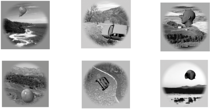
Humans can rapidly visually recognise the actions people around them are engaged in and this ability is important for successful behaviour and social interaction. Isik et al. presented human subjects with 2-second video clips of humans performing actions while measuring brain activity with MEG. The clips comprised 5 actions (walk, run, jump, eat, drink) performed by each of five different actors and video-recorded from each of five different views (only frontal and profile used in MEG). Results show that action can be decoded from MEG signals arising about 200 ms after the onset of the video, with decoding accuracy peaking after about 500 ms and then decaying while the stimulus is still on, with a rebound after stimulus offset. Moreover, decoders generalise across actors and views. The authors conclude that the brain rapidly computes a representation that is invariant to view and actor.

ScreenShot738

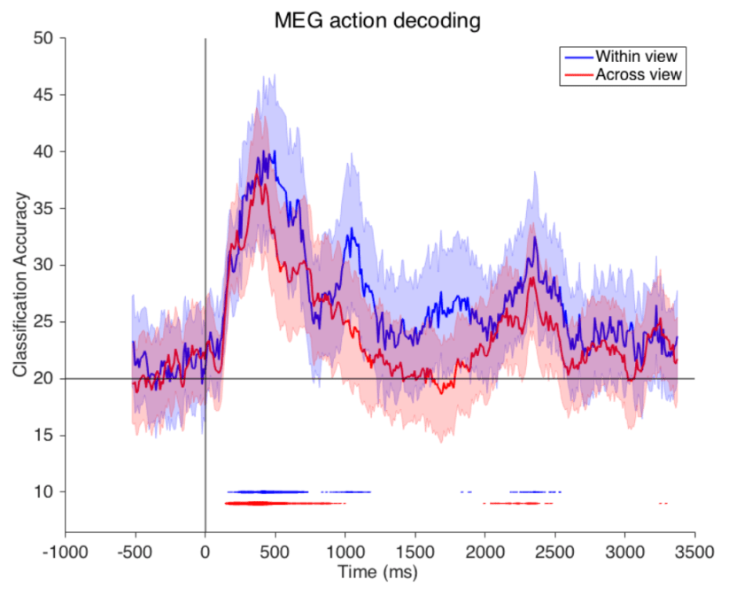
Figure from the paper. Legend from the paper with my modifications in brackets: [Accuracy of action decoding (%) from MEG data as a function of time after video onset]. We can decode [which of five actions was being performed in the video clip] by training and testing on the same view (‘within-view’ condition), or, to test viewpoint invariance, training on one view (0 degrees [frontal, I think, but this should be clarified] or 90 degrees [profile]) and testing on the second view (‘across view’ condition). Results are each [sic] from the average of eight different subjects. Error bars represent standard deviation [across what?]. Horizontal line indicates chance decoding accuracy. […] Lines at the bottom of plot indicate significance with p<0.01 permutation test, with the thickness of the line indicating [for how many of the 8 subjects decoding was significant]. [Note the significant offset response after the 2-s video (whose duration should be indicated by a stimulus bar).]


The rapid view-invariant action decoding is really quite amazing. It would be good to see more detailed analyses to assess the nature of the signals enabling this decoding feat. Of course, 200 ms already allows for recurrent computations and the decodability peak is at 500 ms, so this is not strong evidence for a pure feedforward account.

The generalisation across actors is less surprising. This was a very controlled data set. Despite some variation in the appearance of the actors, it seems plausible that there would be some clustering of the vectors of pixels across space and time (or of features of a low-level visual representation) corresponding to different actors performing the same action seen from the same angle.

In separate experiments, the authors used static single frames taken from the videos and dynamic point-light figures as stimuli. These reduced form-only and motion-only stimuli were associated with diminished separation of actions in the human brain and in model representations, and with diminished human action recognition, suggesting that form and motion information are both essential to action recognition.

I’m wondering about the role of task-related priors. Subjects were performing an action recognition task on this controlled set of brief clips during MEG while freely viewing the clips (though this is not currently clearly stated). This task is likely to give rise to strong prior expectations about the stimulus (0 deg or 90 deg, one of five actions, known scale and positions of key features for action discrimination). Primed to attend to particular diagnostic features and to fixate in certain positions, the brain will configure itself for rapid dynamic discrimination among the five possible actions. The authors present a group-average analysis of eye movements, suggesting that these do not provide as much information about the actions as the MEG signal. However, the low-dimensional nature of the task space is in contrast to natural conditions, where a wider variety of actions can be observed and view, actor, size, and background vary more. The precise prior expectations might contribute to the rapid discriminability of the actions in the brain signals.

The authors model the results in the framework of feedforward processing in a Hubel-and-Wiesel/Poggio-style model that alternates convolution and max-pooling to simulate responses resembling simple and complex cells, respectively. This model is extended here to process video using spatiotemporal filter templates. The first layer uses Gabor filters, higher layers use templates in the first layer matching video clips in the stimulus set. The authors argue that this model supports invariant decoding and largely accounts for the MEG results.

Like the subjects, the model is set up to process the restricted stimulus space. The internal features of the model were constructed using representational fragments from samples from the same parametric space of videos. The exact videos used to test the models were not used for constructing the feature set. However, if I understood correctly, videos from the same restricted space (5 actions, 5 actors, 5 views) were used. Whether the model can be taken to explain (at a high level of abstraction) the computations performed by the brain depends critically on the degree to which the model is not specifically constructed for the (necessarily very limited) 5-action controlled stimulus space used in the study.

As the authors note, humans still outperform computer vision models at action recognition. How does the authors’ own model perform on less controlled action videos? If it the model cannot perform the task on real-world sensory input, can we be confident that it captures the way that the human brain performs the task? This is a concern in many studies and not trivial to address. However, the interpretation of the results should engage this issue.


Strengths

  • Controlled stimulus set: The set of video stimuli (5 actions x 5 actors x 5 views x 26 clips = 3250 2-sec clips) is impressive. Assembling this set is an important contribution to the field. The set is condition-rich (compared to typical stimulus sets used in cognitive neuroscience studies) and seems to strike a good balance between control and realism. This set could be a driver of progress if it were to be used in multiple modelling and empirical studies.
  • Combination of brain-activity measurements and a simple computational model, which provides a useful starting point for modelling the recognition of dynamic actions, as it is minimal and standard in many respects: a feedforward model in the HMAX framework, extended from spatial to spatiotemporal filters.


Weaknesses

  • Controlled stimulus set: The set of video stimuli is very restricted compared to real-world action recognition. For the brain data, this means that subjects might have rapidly formed priors about the stimuli, enabling them to configure their visual systems (e.g. attentional templates, fixation targets) for more rapid recognition of the 5 actions than is possible in real-world settings. This limitation is shared with many studies in our field and difficult to overcome without giving up control (which is a strength, see above). I therefore suggest addressing this problem in the discussion.
  • The model uses features based on spatiotemporal patterns sampled from the same restricted stimulus space. Although non-identical clips were used, the videos underlying the representational space appear to share a lot with the experimental stimuli (same 5 actions, same 5 views, same background?, same actors?). I would therefore not expect this model to work well on arbitrary real-world action video clips. This is in contrast to recent studies using deep convolutional neural nets (e.g. Khaligh-Razavi & Kriegeskorte 2014), where the models were trained without any information about the (necessarily restricted) brain-experimental stimulus set and can perform recognition under real-world conditions.
  • Only one model (in two variants) is tested. In order to learn about computational mechanism, it would be good to test more models.
  • MEG data were acquired during viewing of only 50 of the clips (5 actions x 5 actors x 2 views).
  • Missing inferential analyses: While the authors employ inferential analyses in single subjects and report number of significant subjects, few hypotheses of interest are formally statistically tested. The effects interpreted appear quite strong, so the results described above appear solid nevertheless (interpretational caveats notwithstanding).


Overall evaluation

This is an ambitious study describing results of a well-designed experiment using a stimulus set that is a major step forward. The results are an interesting and substantial contribution to the literature. However, the analyses could be much richer than they currently are and the interpretation of the results is not straightforward. Stimulus-set-induced priors may have affected both the neural processing measured and the model (which used templates from stimuli within the controlled video set). Results should be interpreted more cautiously in this context.

Although feedforward processing is an important part of the story, it is not the whole story. Recurrent signal flow is ubiquitous in the brain and essential to brain function. In engineering, similarly, recurrent neural networks are beginning to dominate spatiotemporal processing challenges such as speech and video recognition. The fact that the MEG data are presented as time courses, revealing a rich temporal structure, and the model analyses are bar graphs illustrates the key limitation of the model.

It would be great to extend the analyses to reveal a richer picture of the temporal dynamics. This should include an analysis of the extent to which each model layer can explain the representational geometry at each latency from stimulus onset.


Future directions

In revision or future studies, this line of work could be extended in a number of ways:

  • Use multiple models that can handle real-world action videos. The authors’ controlled video set is extremely useful for testing human and model representations, and for comparing humans to models. However, to be able to draw strong conclusions, the models, like the humans, would have to be trained to recognise human actions under real-world conditions (unrestricted natural video). In addition, it would be good to compare the biological representational dynamics to both feedforward and recurrent computational models.
  • To overcome the problem of stimulus-set related priors, which make it difficult to compare representational dynamics measured for restricted stimulus sets to real-world recognition in biological brains, one could present a large set of stimuli without ever presenting a stimulus twice to the same subject. Would the action category still be decodable at 150 ms with generalisation across views? Would a feedforward computer vision model trained on real-world action videos be able to predict the representational dynamics?
  • The MEG analyses could use source reconstruction to enable separate analyses of the representational dynamics in different brain regions.
  • It would be useful to have MEG data for the full stimulus set of 5 actions x 5 actors x 5 viewpoints = 125 conditions. The representational geometries could be analysed in detail to reveal which particular action pairs become discriminable when with what level of invariance.


Particular suggestions for improvements of this paper

(1) Present more detailed results

It would be good to see results separately for each pair of actions and each direction of crossdecoding (0 deg training -> 90 deg testing, and 90 deg training -> 0 deg testing). Regarding the former, eating and drinking involve very similar body postures and motions. Is this reflected in the discriminability of these actions?

Regarding, the decoding generalisation across views, you state:

“We decoded by training only on one view (0 degrees or 90 degrees), and testing on a second view (0 degrees or 90 degrees).”

Was the training set exclusively composed on 0 degree (frontal?) and the test set exclusively of 90 degree (side view?), and vice versa? In case the test set contained instances of both views (though of course, not for the same actor and action), results are more difficult to interpret.


(2) Discuss the caveats to the current interpretation of the results

Discuss the question whether priors resulting from subjects understanding of the restricted stimulus set might have affected the processing of the stimuli. Consider the involvement of recurrent computations within 200 ms and discuss the continuing rise of decodability until 500 ms. Discuss the possibility that the model will not generalise to action recognition in the wild.


(3) Test several control models

Can Gabor, HMAX, and deep convolutional neural net models support similarly invariant action decoding? These models are relatively easy to test, so I think it’s worth considering this for revision. Computer vision models trained on dynamic action recognition could be left to future studies.


(4) Test models by comparison of its representations with the brain representations

The computational model is currently only compared to the data at the very abstract level of decoding accuracy. Can the model predict the representations and representational dynamics in detail? It might be difficult to use the model to predict the measured channels. This would require the fitting of a linear model predicting the measured channels from the model units and the MEG data (acquired for only 5 actions x 5 actors x 2 views = 50 conditions) might be insufficient. However, representational dynamics could be investigated in the framework of representational similarity analysis (50 x 50 representational dissimilarity matrices) following Carlson et al. (2013) and Cichy et al. (2014). Note that this approach does not require fitting a prediction model and so appears applicable here. Either approach would reveal the dynamic prediction of the feedforward model (given dynamic inputs) and where its prediction diverges from the more complex and recurrent processes in the brain. This would promise to give us a richer and less purely confirmatory picture of the data and might show the merits and limitations of a feedforward account.


(5) Perform temporal cross-decoding

Temporal crossdecoding (Carlson et al. 2013, Cichy et al. 2014) could be used to more richly characterise the representational dynamics. This would reveal whether representations stabilise in certain time windows, or keep tumbling through the representational space even as stimuli are continuously decodable.


(6) Improve the inferential analyses

I don’t really understand the inference procedure in detail from the description in the methods section.

“We recorded the peak decoding accuracy for each time bin,…”

What is the peak decoding accuracy for each time bin? Is this the maximum accuracy across subjects for each time bin?

“…and used the null distribution of peak accuracies to select a threshold where decoding results performing above all points in the null distribution for the corresponding time point were deemed significant with P < 0.01 (1/100).”

I’m confused after reading this, because I don’t understand what is meant by “peak”.

The inference procedure for the decoding-accuracy time courses seems to lack formal multiple-testing correction across time points. Given enough subjects, inference could be performed with subject as a random effect. Alternatively, fixed-effects inference could be performed by permutation, averaging across subjects. Multiple testing across latencies should be formally corrected for. A simple way to do this is to relabel the experimental events once, compute an entire decoding time course, and record the peak decoding accuracy across time (or if this is what was done, it should be clearly described). Through repeated permutations, a null distribution of peak accuracies can be constructed and a threshold selected that is exceeded anywhere under H0 with only 5% probability, thus controlling the familywise error rate at 5%. This threshold could be shown as a line or as the upper edge of a transparent rectangle that partially obscures the insignificant part of the curve.

For each inferential analysis, please describe exactly what the null hypothesis was, what event-labels are exchangeable under this null hypothesis, and how the null distribution was computed. Also, explain how the permutation test interacted with the crossvalidation procedure. The crossvalidation should ideally generalise to new stimuli and label permutation be wrapped around this entire procedure.

“Decoding analysis was performed using cross validation, where the classifier was trained on a randomly selected subset of 80% of data for each stimulus and tested on the held out 20%, to assess the classifier’s decoding accuracy.”

Does this apply only to the within-view decoding? In the critical decoding analysis with generalisation across views, it cannot have been 20% of the data in the held-out set, since 0-deg views were used for training and 90-deg views for testing (and vice versa). If only 50% of the data were used for training there, why didn’t performance suffer given the smaller training set compared to the within-view decoding?

It would also be good to have estimates and inferential comparisons of the onset and peak latencies of the decoding time courses. Inference could be performed on a set of single-subject latency differences between two conditions modelling subject as a random effect.


(7) Qualify claims about biological fidelity of the model

The model is not really “designed to closely mimic the biology of the visual system”, rather its architecture is inspired by some of the features of the feedforward component of the visual hierarchy, such as local receptive fields of increasing size across a hierarchy of representations.


(8) Open stimuli and data

This work would be especially useful to the community if the video stimuli and the MEG data were made openly available. To fully interpret the findings, it would also be good to be able to view the movie clips online.


(9) Further clarify the title

The title “Fast, invariant representation for human action in the visual system” is somewhat unclear. What is meant are representations of perceived human actions, not representations for action. “Fast, invariant representation of visually perceived human actions” would be better, for example.


(10) Clarify what stimuli MEG data were acquired for

The abstract states “We use magnetoencephalography (MEG) decoding and a computational model to study action recognition from a novel dataset of well-controlled, naturalistic videos of five actions (run, walk, jump, eat, drink) performed by five actors at five viewpoints.” This suggests that MEG data were acquired for all these conditions. The methods section clarifies that MEG data were only recorded for 50 conditions (5 actions x 5 actors x 2 views). Here and in the legend of Fig. 1, it would be better to use the term “stimulus set” in place of “data set”.


(11) Clarify whether subjects were fixating or free viewing

Were subjects free viewing or fixating? This should be explicitly stated and the choice motivated in either case.


(12) Make figures more accessible

The figures are not optimal. Every panel showing decoding results should be clearly labelled to state what variables the crossvalidation procedure tested for generalisations across. For example, a label (in the figure itself!) could be: “decoding brain representations of actions with invariance to actor and view”. The reader shouldn’t have to search in the legend to find this essential information. Also every figure should have a stimulus bar depicting the period of stimulus presence. This is important especially to assess stimulus-offset-related effects, which appear to be present and significant.

Fig. 3 is great. I think it would be clearer to replace “space-time dot product” with “space-time convolution”.


(13) Clarify what the error bars represent

“Error bars represent standard deviation.”

Is this the standard deviation across the 8 subjects? Is it really the standard deviation or the standard error?


 (14) Clarify what we learn from the comparison between the structured and the unstructured model

For the unstructured model, won’t the machine learning classifier learn to select random combinations that tend to pool across different views of one action? This would render the resulting system computationally similar.