A cortico-thalamic model of multi-scale incremental feature binding

Our retinae sample the images in our eyes discretely, conveying a million local measurements through the optic nerve to our brains. Given this piecemeal mess of signals, our brains infer the structure of the scene, giving us an almost instant sense of the geometry of the environment and of the objects and their relationships.

We see the world in terms of objects. But how our visual system defines what an object is and how it represents objects is not well understood. Two key properties thought to define what an object is in philosophy and psychology are spatiotemporal continuity and cohesion (Scholl 2007). An object can be thought of as a constellation of connected parts, such that if we were to pull on one part, the other parts would follow along, while other objects might stay put. Because the parts cohere, the region of spacetime that corresponds to an object is continuous. The decomposition of the scene into potentially movable objects is a key abstraction that enables us to perceive, not just the structure and motion of our surroundings, but also the proclivities of the objects (what might drop, collapse, or collide) and their affordances (what might be pushed, moved, taken, used as a tool, or eaten).

An important computational problem our visual system must solve, therefore, is to infer what pieces of a retinal image belong to a single object. This problem has been amply studied in humans and nonhuman primates using behavioral experiments and measurements of neural activity. A particular simplified task that has enabled highly controlled experiments is mental line tracing. A human subject or macaque fixating on a central cross is presented with a display of multiple curvy lines, one of which begins at the fixation point. The task is to judge whether a peripheral red dot is on that line or on another line (called a distractor). Behavioral experiments show that the task is easy to the extent that the target line is short or isolated from any distractors. Adding distractor lines in the vicinity of the target line to clutter up the scene and making the target line long and curvy makes the task more difficult. If the target snakes its way through complex clutter closeby, it is no longer instantly obvious where it leads and attention and time are required to judge whether the red dot is on the target or on a distractor line.

Our reaction time is longer when the red dot is farther from fixation along the target line. This suggests that the cognitive process required to make the judgment involves tracing the line with a sequential algorithm, even when fixation is maintained at the central cross. However, the reaction time is not in general linear in the distance, measured along the line, between the fixation point and the dot, as would be predicted by sequential tracing of the line at constant speed. Instead, the speed of tracing is variable depending on the presence of distracting lines in the vicinity of the current location of the tracing process along the target line. Tracing proceeds more slowly when there are distracting lines close by and more quickly when the distracting lines are far away.

The hypothesis that the primate visual system traces the line sequentially from the fixation point is supported by seminal electrophysiological experiments by Pieter Roelfsema and colleagues, which have shown that neurons in early visual cortex that represent particular pieces of the line emanating from the fixation point are upregulated in sequence, consistent with a sequential tracing process. This sequential upregulation of activity of neurons representing progressively more distal portions of the line is often interpreted as the neural correlate of attention spreading from fixation along the attended line during task performance.

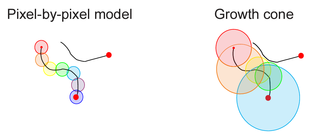
The variation in speed of the tracing process can be explained by the attentional growth-cone hypothesis (Pooresmaeili & Roelfsema 2014) which posits that attention spreads not only in the primary visual cortex but also at higher levels of cortical representation. This hypothesis can explain the variation in tracing speed: At higher levels of cortical visual representation, neurons have larger receptive fields and offer a coarser-scale summary of the image, enabling the tracing to proceed at greater speed along the line in the image. In the absence of distractors, tracing can proceed quickly at a high-level of representation. However, in the presence of distractors, the higher-level representations may not be able to resolve the scene at a sufficient grain, and tracing must proceed more slowly in lower-level representations.

Higher-level neurons are more likely to suffer from interference from distractor lines within their larger receptive fields. If a distractor line is present in a neuron’s receptive field, the neuron may not respond as strongly to the line being traced, effectively blocking the path for sequential tracing in the high-level representation. However, tracing can continue – more slowly – at lower levels, where receptive fields are small enough to discern the line without interference.

Detail from Fig. 6 in Pooresmaeili et al. (2014) illustrating the single-scale tracing model (left) and the growth-cone model (right), in which the attentional label is propagated from the fixation point (small red dot) at all levels of representation where receptive fields (circles) do not overlap with the distractor curve. Tracing proceeds rapidly at coarse scales (orange, blue) where the target line is far from the distractor and slowly at fine scales (yellow, green) where the target curve comes close to the distractor.

Now Schmid & Neumann (pp2024) offer a brain-computational model explaining in detail how this multiscale algorithm for attentional selection of the line emanating from the fixation point might be implemented in the primate brain. They describe a mechanistic model and demonstrate by simulation that it can explain how mental line tracing might be implemented in the primate brain. 

Pyramidal neurons at multiple levels of the visual hierarchy (corresponding to cortical areas V1, V2, V4) detect local oriented line segments on the basis of the bottom-up signals arriving at their basal dendritic integration sites. These line segments are pieces of the target and distractor lines, represented in each area at a different scale of representation. The pyramidal neurons also receive lateral and top-down input providing contextual information at their apical dendritic integration sites, enabling them to sense whether the line segment they are representing is part of a longer continuous line.

The attentional “label” indicating that a neuron represents a piece of the target line is encoded by an upregulation of the activity of the pyramidal neurons, consistent with neural recording results from Roelfsema and colleagues (1998). The upregulation of activity, i.e. the attention label, can spread laterally within a single area such as V1. Connectivity between neurons representing approximately collinear line segments implements an inductive bias that favors interpretations conforming to the Gestalt principle of good continuation. However, the upregulation will spread only to pyramidal neurons that (1) are activated by the stimulus, (2) receive contextual input from pyramidal neurons representing approximately collinear line segments, and (3) receive thalamic input indicating the local presence of the attentional marker. 

Each step of propagation is conditioned on the conjunction of these three criteria. The neural computations could be implemented exploiting the intracellular dynamics in layer-5 pyramidal neurons, where dendritic inputs entering at apical integration sites cannot drive a response by themselves but can modulate responses to inputs entering at basal integration sites. An influential theory suggests that contextual inputs arriving at the apical dendritic integration sites modulate the response to bottom-up stimulus inputs arriving at the basal dendritic integration sites (Larkum 2013, BrainInspired podcast). Schmid and Neumann’s model further posits that the apical inputs are gated by thalamic inputs (Halassa & Kastner 2017), implementing a test of the third criterion for propagation of the attentional label.

The attentional label is propagated locally from already labeled pyramidal neurons to pyramidal neurons at all levels of the visual hierarchy that represent closeby line segments sufficiently aligned in orientation to be consistent with their being part of the target line. To enable the coarser-scale representations in higher cortical areas to speed the process, neurons representing the same patch of the visual field at different scales are connected through thalamocortical loops. Through the thalamus, each level is connected to all other levels, enabling label propagation to bypass the stages of the hierarchy. The thalamic component (possibly in the pulvinar region of the visual thalamus) represents a map of the labeled locations, but not detailed orientation information.

Imagine a mechanical analogy, in which tube elements represent local segments of the lines. The stimulus-driven bottom-up signals align the orientations of the tube elements with the orientations of the line segments they represent, so the tube elements turn to form long continuous tunnels depicting the lines. A viscous liquid is injected into the tube element representing the fixation point and spreads. Adjacent tube elements need to be aligned for the liquid to flow from one into the other. In addition, there are valves between the tube elements, which open only in the presence of thalamic input. Importantly, the viscous liquid can flow not only at the V1 level of representation, where the tube elements represent tiny pieces of the lines and the viscous liquid needs to flow through many elements to reach the end of the line. Rather, the liquid can also take shortcuts through higher-level representations, where long stretches of the line are represented by few tube elements. This enables the liquid to reach the end of the line much more quickly – to the extent that there are stretches sufficiently isolated from the distractors for coarse-scale representation at higher levels of the hierarchy.

Since the information about (1) the presence of oriented line segments, (2) their compatibility according to the Gestalt principle of good continuation, and (3) the attentional label are all available in the cortical hierarchy, a growth-cone algorithm could be implemented without thalamocortical loops. However, Schmid and Neumann argue that the non-orientation-specific thalamic representation reduces the complexity of the circuit. Fewer connections are required by decomposing the question “Are there upregulated compatible signals in the neighborhood?” into two simpler questions: “Are there compatible signals in the neighborhood?” (answered by cortex) and “Are there upregulated signals in the neighborhood?” (answered by the thalamic input). Because there could be compatible signals in the neighborhood that are not upregulated, and upregulated signals that are not compatible, yeses to both questions of the decomposition do not in general imply a yes to the original question. However, if we assume that there is only one line segment per location, then two yeses do imply a yes to the original question.

Schmid and Neumann argue that thalamic label map enables a simpler circuit that works in the simulations presented, even tracing a line as it crosses another line without spillover. We wonder if, in addition to requiring fewer connections, the thalamic label map might have functional advantages in the context of a system that must be able to perform not just line tracing but many other binding tasks, where the thalamus might have the same role, but the priors defining compatibility could differ.

Why is this model important? Line tracing is a type of computational problem that is prototypical of vision and yet challenging for both of our favorite modes of thinking about visual computations: deep feedforward neural networks and probabilistic inference. These two approaches (discriminative and generative to a first approximation) form diametrically opposed corners in a vast space of visual algorithms that has only begun to be explored (Peters et al. pp2023). Line tracing is a simple example of a visual cognition task that can be rendered intractable for both approaches by making the line snaking its way through the clutter sufficiently long and the clutter sufficiently close and confusing. Feedforward deep neural networks have trouble with this kind of problem because there are no hints in the local texture revealing the long-range connectivity of the lines. The combinatorics creates too rich a space of possible curves to represent with a hierarchy of features in a neural network. Although any recurrent computation (including the model of Schmid and Neumann and a recent line tracing model from Linsley & Serre, 2019) can be unfolded into a feedforward computational graph, the feedforward network would have to be very deep, and its parameters might be hard to learn without the inductive bias that iterating the same local propagation rule is the solution to the puzzle (van Bergen & Kriegeskorte 2020). From a probabilistic inference perspective, similarly, the problem is likely intractable in its general form because of the exponential number of possible groupings we would need to compute a posterior distribution over.

By assuming that we can be certain about the way things connect locally, we can avoid having to maintain a probability distribution over all possible line continuations from the fixation point. Binarizing the probabilities turns the problem into a region growing (or graph search) problem requiring a sequential procedure, because later steps depend on the result of earlier steps.

Schmid and Neumann’s paper describes how the previously proposed growth-cone algorithm, which solves an important computational challenge at the heart of visual cognition (Roelfsema 2006), might be implemented in the primate brain. The paper seriously engages both the neuroscience (at least at a qualitative level) and the computational problem, and it connects the two. The authors simulate the model and demonstrate its predictions of the key behavioral and neurophysiological results from the literature. They use model-ablation experiments to establish the necessity of different components. They also describe the model at a more abstract level: reducing the operations to sequential logical operations and systematically considering different possible implementations in a circuit and their costs in terms of connections. This resource-cost perspective deepens our understanding of the algorithm and reveals that the proposed model is attractive not only for its consistency with neuroanatomical, neurophysiological, and behavioral data, but also for the efficiency of implementation in a physical network.

Strengths

  • Offers a candidate explanation for how an important cognitive function might be implemented in the primate brain, using an algorithm that combines parallel computation, hierarchical abstraction, and sequential inference.
  • Motivated by a large body of experimental evidence from neurophysiological and behavioral experiments, the model is consistent with primate neuroanatomy, neural connectivity, neurophysiology, and subcellular dynamics in multi-compartment pyramidal neurons.
  • Describes a class of related algorithms and network implementations at an abstract level, providing a deeper understanding of alternative possible neural mechanisms that could perform this cognitive function and their network complexity.

Weaknesses

  • The model operates on a toy version of the task, using abstracted stimuli with few orientations and predefined Gabor filter banks as model representations, rather than more general visual representations learned from natural images. An important question is to what extent the algorithm will be able to perform visual tasks on natural images. Given the complexity of the paper as is, this question should be considered beyond the scope, but related work connecting these ideas to computer vision could be discussed in more detail.

Major suggestions

(1) Illustrate the computational mechanism and operation of the model more intuitively. In Fig. 1b, colors code for the level of representations. It would therefore be better to not use green to code for the selection tag. Thicker black contours or some other non-color marker could be used. It is also hard to see that the no-interference and the interference cases have different stimuli. Only the bottom panels with the stimuli show a slight difference. The top panels should be distinct as well since different neurons would be driven by the two stimuli. Alternatively, you could consider using only one stimulus, where the distractor distance variation is quite pronounced, but showing time frames to illustrate the variation of the speed of the progression of attentional tagging.

(2) Discuss challenges in scaling and calibrating the model for application to natural continuous curves. The stimuli analyzed have only a few orientations with sudden transitions from one to the other. Would the model as implemented also work for continuous curves such as those used in the neurophysiological and behavioral experiments or would a finer tiling of orientations be required? Under what conditions would attention spill over to nearby distractor curves? It would be good to elaborate on the roles of surround suppression, inhibition among detectors, and the excitation/inhibition balance. 

(3) Discuss challenges in scaling the model to computer vision tasks on natural images. To be viable as brain-computational theories, models ultimately need to scale to natural tasks. Please address the challenges of extending the model for application to natural images and computer-vision tasks. This will likely require the representations to be learned through backpropagation. The cited complementary work by Linsley and Serre on the pathfinder task using horizontal gated recurrent units and incremental segmentation for computer vision is relevant here and deserves to be elaborated on in the Discussion. In particular, do the growth-cone model and your modeling results suggest an alternative neural network architecture for learning incremental binding operations?

Minor suggestions

(1) Please make sure that the methods section contains all the details of the model architecture needed for replication of the work. Much of the math is described well. But some additional technical details on maps and connectivity may be needed. What are the sizes of the maps? What do they look like for a given input? Do they appear like association fields? What is the excitatory and inhibitory connectivity as a function of spatial locations and orientations of the source and target unit?

(2) Discuss how the model relates to the results of Chen et al. (2014) who described the interplay between V1 and V4 during incremental contour integration on the basis of simultaneous recordings in monkeys.

(3) Although the paper is well-written and clear, the English is a bit rocky throughout with many grammatical errors and some typos. These could be fixed using a proofreader or suitable software. 

– Nikolaus Kriegeskorte & Hossein Adeli

References

Chen M, Yan Y, Gong X, Gilbert CD, Liang H, Li W (2014) Incremental integration of global contours through interplay between visual cortical areas Neuron.

Halassa MM, Kastner S. Thalamic functions in distributed cognitive control. Nature neuroscience. 2017 Dec;20(12):1669-79.

Lamme VA, Roelfsema PR (2000) The distinct modes of vision offered by feedforward and recurrent processing Trends in Neurosciences.

Larkum M. A cellular mechanism for cortical associations: an organizing principle for the cerebral cortex. Trends in neurosciences. 2013 Mar 1;36(3):141-51.

Larkum ME, Zhu JJ, Sakmann B (1998) A new cellular mechanism for coupling inputs arriving at different cortical layers Nature.

Linsley D, Kim J, Veerabadran V, Serre T (2019) Learning long-range spatial dependencies with horizontal gated-recurrent units NeurIPS. arxiv.org/abs/1805.08315.

Peters B, Kriegeskorte N (2021)  Capturing the objects of vision with neural networks. Nature human behaviour Nature Human Behavior.

Peters B, DiCarlo JJ, Gureckis T, Haefner R, Isik L, Tenenbaum J, Konkle T, Naselaris T, Stachenfeld K, Tavares Z, Tsao D, Yildirim I, Kriegeskorte N (under review) How does the primate brain combine generative and discriminative computations in vision? CCN GAC paper. arXiv preprint arXiv:2401.06005.

Pooresmaeili A, Roelfsema PR (2014) A growth-cone model for the spread of object-based attention during contour grouping Current Biology

Roelfsema PR, Lamme VA, Spekreijse H (1998) Object-based attention in the primary visual cortex of the macaque monkey Nature

Roelfsema PR (2006) Cortical algorithms for perceptual grouping Annu Rev Neurosci.

Scholl BJ (2007) Object persistence in philosophy and psychology Mind & Language.

van Bergen RS, Kriegeskorte N (2020) Going in circles is the way forward: the role of recurrence in visual inference Current Opinion in Neurobiology.

Neural net models may lack crucial mechanisms (not just data) to acquire human-like robustness of visual recognition

Neural network (NN) models have brought spectacular progress in computer vision and visual computational neuroscience over the past decade, but their performance, until recently, was quite brittle: breaking down when images are compromised by occlusions, lack of focus, distortions, and noise — sources of nuisance variation that human vision is robust to. The robustness of recognition has substantially improved in recent models with extensive training and data augmentation.

Extensive visual experience also drives the development of human visual abilities. Humans, too, experience a vast number of visual impressions, many of them compromised and all of them embedded in a context of previous visual impressions and information from other sensory modalities, including audition, that can constrain the interpretation of the scene and drive visual learning. Do state-of-the-art robust NN models provide a good model of robust recognition in humans, then?

A new paper by Huber et al. (pp2022) suggests that a training-based account of the robustness of human vision, along the lines of the recent advances in getting NN models to be more robust through extensive training, is uncompelling. Current NN models, they argue, lack some essential computational mechanisms that enables the human brain to achieve robustness with less visual experience.

The authors measured recognition abilities in 146 children and adolescents, aged 4-15, and found that even the 4-6 year-olds outperformed current NN models at recognizing images robustly under substantial local distortions (so called eidolon distortions). They argue that back-of-the-envelope estimates of the amount of visual experience suggest that humans achieve greater robustness with less training data. The human visual system must have some additional mechanism in place that current NN models lack.

One possibility is that human vision has mechanisms to perceive the global shape of objects more robustly than current NN models. Using ingenious shape-texture-cue-conflict stimuli, which they introduced in earlier work, the authors show that the well-known human bias in favor of classifying objects by their shape is already present in the 4-6 year olds. Testing the models with the shape-texture-cue-conflict stimuli showed, by contrast, that even the most extensively trained and robust NN models rely much more strongly on texture than on shape.

To compare the amount of visual experience between humans and models, the authors offer a back-of-the-envelope calculation (their appropriate term), in which they quantify human visual experience at a given age in the currency of NN models: number of images. They use estimates of the number of waking hours across childhood and of the number of fixations per second. One fixation is assumed as roughly equivalent to a training image. According to such estimates, the best model (SWAG) requires about an order of magnitude more data to reach human-level robustness.

This calculation and the corresponding figure are interesting because they provide a starting point for an important discussion. However, the estimate suggesting an order of magnitude difference in the amount of data required could easily be off by more than an order of magnitude.

More importantly, the estimate (though it is an interesting starting point) is fundamentally flawed and should be accompanied by more critical arguments. Human visual experience is temporally continuous and dependent and therefore cannot meaningfully be quantified in terms of a number of training images or exposures (counting multiple exposures to augmented versions of the same image across epochs).

It is also unclear why fixations should be equated to images. We see a dynamic world evolve at a rate much faster than the rate of fixations. Moreover, fixations are actively chosen, so their information content may be greater than that of a similar number of i.i.d. samples. (This could count as one of the qualitative differences between primate vision and current NN models: Primate visual recognition is active perception, and visual learning is active learning: The animal makes its own curriculum and this could contribute to its learning more from less data.)

A simpler calculation (and the one I couldn’t resist typing into my calculator before getting to the authors’) would equate frames (perhaps 10 per second?) to training images. Of course, frames are not a well-defined concept, either, in the context of human visual experience and, at 10 frames per second, successive frames are highly dependent. However, temporal dependency may be a critical feature, helping rather than hurting visual learning. At 10 frames per second, the calculation yields an estimate surprisingly close to the “amount of visual experience” of the state-of-the-art models.

Another reason why comparing visual experience between models and humans is inherently difficult concerns the quality, rather than the quantity, of the visual input. The out-of-distribution generalization challenge is not (and cannot readily be) matched between humans and models. Human visual experience may include more distorted inputs due to physical processes in the world such as rain and glass obscuring the scene as well as due to optical imperfections of our eyes. As a result, human visual experience may provide better training for generalizing to the eidolon distortions than the training sets used for the most extensively trained models (SWAG and SWSL).

The claims relating to the comparison of the “amount of visual experience” between humans and models should be tempered in revision and more critically discussed with a view to directions for future studies. It would also be good to add statistical inference to demonstrate that the reported effects generalize across stimuli and subjects. The error consistency analysis is important. However, I find the boxplots hard to interpret. It would be great to see inferential comparisons between different DNNs, where currently DNNs are lumped together despite the fact that there appears to be little inter-DNN error consistency.

The authors are almost certainly correct that current NN models lack essential computational mechanisms. However, I’m not sure if the estimates of the amount of visual experience in the current version of the paper provide strong evidence for the greater data efficiency of human vision.

Overall this paper describes an important, carefully designed and executed study and offers a unique open-science human developmental cross-sectional data set on object-recognition robustness for further systematic analyses. The use of state-of-the-art models and the careful discussion of the state of the field make this a great contribution.

Strengths

  • Important comprehensive novel behavioral data set
  • Challenge of experimenting with kids of different ages met with carefully designed and executed experiment
  • All code and data available via github
  • Comparison to four NN models that represent the state of the art at out-of-distribution robust recognition and span four orders of magnitude of training-set size (1M, 10M, 100M, 1B images)
  • Interesting discussion highlighting the difficulty of quantifying and comparing “the amount of visual experience” between models and humans

Weaknesses

  • The “back-of-the-envelope” calculation on the amount of visual experience is not just a very rough approximation, but conceptually flawed: Human visual experience is temporally continuous and dependent, and thus cannot be approximately quantified in terms of a number of i.i.d. images.
  • The out-of-distribution generalization challenge is not (and cannot readily be) matched between humans and models. Human visual experience may provide better training for generalizing to the eidolon distortions than the training sets used for the most extensively trained models (SWAG and SWSL).
  • Hypotheses are not evaluated by statistical inference to generalize to the populations of subjects and stimuli.
  • Age may be confounded by ability to attend on the task and by factors related to participant recruitment. (However, this reflects inherent difficulties of the research not shortcomings of this particular study.)
  • Model architecture is not varied systematically and independently of training regime. (However, this is very hard to achieve given the scale of the models and training sets, and they key conclusions appear compelling despite this shortcoming.)

Minor notes

“not only subjective effortless but objectively often impressive” typo: should be “subjectively”. Also: impressiveness is inherently subjective.

knive -> knife

Fig. 4: Panel labels (a), (b) should be bigger, bold and above, not below the panels. The top should be a.

Fig. 4a: The logarithmic horizontal axis tick labels are inconsistent between the panels.

Fig. 5 (left): accuracy delta should be described “4-6 year-olds minus adults”, not vice versa

Does our proprioceptive system try to recognize our own actions?

Proprioception is our sense of the motion and posture of our own body. This sixth sense uses signals from receptors in the joints, tendons, muscles, and skin that measure forces and degrees of extension. These receptors enable us to sense, for example, the posture of our body as we wake from sleep. They also provide feedback signals that help us precisely control our limbs, for example during handwriting.

Feedback is thought to be essential to motor control, enabling the controller in our brains to rapidly adapt to the unexpected. The unexpected may include changes in the environment (like something  pushing our hand that we didn’t see coming), changes in our bodies (such as muscle fatigue or injury), and shortcomings of the motor program (such as a lack of precision or a badly planned limb trajectory). Feedback can come from vision and even audition, but proprioception provides an essential additional feedback path that informs us directly about the motion and posture of our limbs, and any forces on them.

How does feedback control work in the human motor system? I want to write a ‘k’, but there are forces on my limbs resulting from the friction of chalk on this particular blackboard. Also, my muscles are recovering from tennis practice this morning, and I haven’t used chalk on a blackboard in years.

If the goal is to write a ‘k’, I have some flexibility. I am committed, not to a precise trajectory, but to a more abstractly defined objective: to write a legible ‘k’. This suggests that feedback processing should evaluate to what extent I am succeeding at the action, not at tracing out a particular trajectory. Does what I’m actually doing look like writing a ‘k’?

In a new paper, Sandbrink et al. (pp2022) report on simulations of the human musculoskeletal system and neural network models that suggest that the tuning properties of neurons in somatosensory cortex (S1) can be explained by assuming that the objective of the proprioceptive system is to recognize the action being performed.

They used recorded traces of a person writing lower-case letters to simulate the responses of muscle spindles sensing the lengths and velocities of muscles in the human arm as would be present if the hand were moved passively along these trajectories. The physical simulation uses a 3D model of the human arm with two parameters for the direction of the upper arm and two more for the direction of the lower arm. These four parameters are inferred by inverse kinematics from the hand trajectories tracing each letter in a variety of vertical and horizontal planes. A 3D muscle model then enables the authors to compute the expected spindle responses that reflect the lengths and velocities of 25 relevant upper arm muscles.

The authors then trained neural network models of proprioceptive processing that took the simulated muscle spindle signals as input. The neural net architectures included one that first integrates information over the muscle spindles and then across time (“spatial-temporal”), one that integrated across muscle spindles and time simultaneously (“spatiotemporal”), and a recurrent long-short-term-memory model.

Each architecture was trained on two objectives: to decode the trajectory (i.e. the position of the hand tracing a letter as a function of time) or to recognize the action (i.e. the letter being traced). The two objectives correspond to two hypotheses about the function of proprioceptive processing: To inform the feedback controller about either the current position of the hand or the letter being drawn.

The models trained to recognize the action developed tuning more consistent with what is known about the tuning of neurons in primary somatosensory cortex in primates. In particular, direction tuning with roughly equal numbers of units preferring each direction emerged in middle layers of the neural network models trained to recognize the action, similar to what has been observed in primate neural recordings. Direction tuning is already present in the muscle-spindle signals, but the spindle signals do not uniformly represent the directions.

The task-optimization approach to neural network modeling is inspired by work in vision, where neural networks trained on the task of image classification explained responses to novel images in populations of neurons in the inferior temporal cortex. This result suggested a tentative answer to the why question: Why do inferior temporal neurons exhibit the response profiles and representational geometry they exhibit? Because their function (or one of their functions) is to recognize the objects in the images. Here, similarly, the authors address a why question with task-optimized neural network models: Why do somatosensory cortical neurons exhibit the types of tuning that have been reported in the literature?

The function of proprioception, of course, is not for the brain to recognize which letter it is trying to write. It already knows that. The function is to sense how the current trajectory – the actual, not the intended one – differs from, say, a legible “k” (if that was the intention), and to map from that difference to a modification vector that will improve the outcome.

Why is action decoding relevant for performing the action? A key reason may be that the goal is not to produce a fixed trajectory, but to produce a legible ‘k’. A legible ‘k’ is not a single trajectory, but a class of trajectories containing an infinity of viable solutions. If someone nudged my arm while writing, adaptive feedback control should not attempt to return me to the originally intended trajectory, but to a new trajectory that traces the most legible ‘k’ that is still in the cards, which may be a different style of ‘k’ than I originally intended.

The paper contributes a useful data set for training models and a qualitative comparison of models to real neurons in terms of tuning properties. It would be good, in follow-up studies, to directly test to what extent each of the models can quantitatively predict either single-neuron responses or population representational geometries, as has been done in vision, and to perform statistical comparisons between models.

Importantly, this paper develops the idea of combining simulations body and brain, of the musculoskeletal system and the processing of control-related signals in the nervous system, which provides a very exciting direction for future research.


Strengths

  • The paper introduces a highly original research program that marries simulation of the musculoskeletal system and neural network modelling to predict neural representations in the proprioceptive pathway.
  • The authors performed an architecture search and trained multiple instances of different neural network architectures with each of two objectives.
  • The paper includes comprehensive analyses of the proprioceptive representations from the simulated muscle-spindle signals through the layers of the models. These analyses characterize unit tuning, linear decodability, and representational similarity.
  • The results suggest an explanation for the direction tuning with a roughly uniform distribution of the units’ direction preferences that has been reported previously for neurons in the primate primary somatosensory (S1) cortex.
  • If the simulated muscle-spindle data set, models, and analysis code were shared along with the published paper, this work could form the basis for quantitative model evaluation and further model development.

Weaknesses

  • The models are qualitatively evaluated by comparison of model unit tuning to what is known about the tuning of neurons in somatosensory cortex. Follow-up studies should quantitatively evaluate the models by inferential analyses of their ability to predict measured responses.
  • The two training objectives differ in multiple respects, making it difficult to assess what the necessary requirements are for the emergence of representations similar to primate S1. Decoding the hand position may be too simple, but what about decoding velocity, or trajectory descriptors such as curvature? There may be a middle ground between trajectory decoding and action recognition that also leads to the emergence of tuning properties as found in primate S1.

What type of linear or nonlinear model should we use to map between brain-representational models and measured neural responses?

Ivanova, Schrimpf, Anzellotti, Zaslavsky, Fedorenko, and Isik (pp2021) discuss whether mapping models should be linear or nonlinear. This paper is part of a Cognitive Computational Neuroscience 2020 Generative Adversarial Collaboration, with the goal to resolve an important controversy in the field.

The authors usefully define the term mapping model in contradistinction to models of brain function. A mapping model specifies the mapping between a model of brain function (some brain-representational model) and brain-activity measurements. A mapping model can relate brain-activity measurements to different types of brain-representational model: (1) descriptions of the stimuli, (2) descriptions of behavioral responses, (3) activity measurements in other brains or other brain regions, or (4) the units in some layer of a neural network model. Moreover, mapping models can operate in either direction: from the measured brain activity to the features of the representational model (decoding model) or from the model features to the measured brain activity (encoding model). Figures 1 and 2 of the paper very clearly lay out these important distinctions.

To begin addressing the question what mapping models should be used the authors consider three desiderata: (1) predictive accuracy, (2) interpretability, and (3) biological plausibility. Predictive accuracy tends to favor more complex and nonlinear models (assuming we have enough data for fitting), whereas simpler and linear models may be easier to interpret in general. Biological plausibility would appear to be irrelevant if the mapping model is not considered a model of brain function. However, in the context of an encoding model, for example, we may want the mapping model to capture physiological processes such as the hemodynamics and nonphysiological processes such as the averaging in voxels, neither of which may be considered part of the brain-computational process that is the ultimate target of our investigation.

The authors make many reasonable points about linear and nonlinear mapping models and conclude by suggesting that rather than the linear/nonlinear distinction, we should consider more general notions of the complexity of the mapping model. They suggest that researchers consider a range of possible mapping models and estimate their complexity. They discuss three measures of complexity: the number of parameters, the minimum description length, and the amount of fitting data needed for a model to achieve a given level of predictive accuracy.

The paper makes a good contribution by beginning a broader discussion about mapping models and putting the pieces of the puzzle on the table. However, a problem is that the arguments are not developed in the context of clearly defined research goals. The three desiderata (predictive accuracy, interpretability, and biological plausibility) are referred to as “goals” in the paper and further differentiated in Fig. 3:

  • predictive accuracy
    • compare competing feature sets
    • decode features from neural data
    • build maximally accurate models of brain activity
  • interpretability
    • examine individual features
    • test representational geometry
    • interpret feature sets
  • biological plausibility
    • incorporate physiological properties of the measurements
    • simulate downstream neural readout

A lot of thought clearly went into this structure, which serves to enable insights at a more general level about the mapping model: for all cases where we desire biological plausibility, interpretability, or predictive accuracy. However, the cost of this abstraction is too great. Arguments for particular choices of mapping model are compelling only in the context of more specifically defined research goals that actually motivate researchers to conduct studies.

Neither the three top-level desiderata, nor the more specific objectives really capture the goals that motivate researchers. We don’t do studies to achieve “predictive accuracy”. Rather our goal may be to adjudicate among different computational models that implement hypotheses about brain information processing. The models’ predictive accuracy is used as a performance statistic to inferentially compare the models.

The goal to compare brain-computational models, for example, is difficult to localize in the list. It is related to “comparing competing feature sets”, “building accurate model of brain activity”, “biological plausibility”, and “testing representational geometry”, but each of these captures only part of the goal to test brain-computational models.

On a similar note, I would argue that “decoding features” is not a research goal. The relevant research goal could be defined as “testing a brain region for the presence of particular information” or “testing whether particular information is explicitly encoded in a brain region”.

It would help to start with research goals that really capture scientists motivation for conducting studies that use mapping models, and then to discuss the merits of particular choices of mapping model in each of these contexts. Some research goals are: testing if certain information is present in a region, testing if it is present in a particular format, adjudicating among representational models, and adjudicating among brain-computational models. Starting with these would make it easier for the reader to follow, and would enable the authors to make some of the arguments already made (e.g. that testing for the presence of information can benefit from nonlinear decoders) more compellingly. It might also lead to additional insights.

An important question is how this CCN Generative Adversarial Collaboration (GAC) can lead to progress beyond this position paper. One topic for further study is the suggestion made at the end that a variety of mapping models should be considered and compared in terms of their complexity and predictive accuracy. This suggestion seems potentially important, but would need (1) careful motivation in the context of particular research goals and (2) more research that develops and validates methods for actually exploring the space of mapping models with flexible regularization. This could be the basis for the aim of the GAC to lead to new research that resolves some challenge or controversy.

Specific comments

Is it that simple? Linear mapping models in cognitive neuroscience

When I read the title, I want to ask back: Is what exactly that simple? What is it? I might interpret the question in the context of the research goal I most care about (adjudicating among brain-computational theories). In that context, I guess, I’m on team linear. (I want to confine nonlinearities to the brain-computational model.) But the vagueness entailed by the absence of explicit research goals starts right there in the title.

If the features are pixels, the answer might be different than if the features are semantic stimulus descriptors (e.g. nonlinear for pixels, linear for semantic features if we are looking for their explicit representation in the brain). If the brain responses are single-cell recordings, the answer might be different than if the brain responses are fMRI voxels (in the latter case, we may want the mapping model to capture averaging within voxels). If the goal is to reveal whether particular information is present in a brain region, we might want to use a nonlinear decoding analysis. If the goal is to reveal whether particular information is explicitly encoded in the sense of linear decodability, we might want to use a linear decoding analysis. If the goal is to test a brain-computational model of perception, the answer will depend on whether the mapping model is supposed to serve solely the purpose of mapping model representations to brain representations, or whether it is supposed to be interpreted as part of the brain-computational model (i.e. whether we intend to use the brain-activity data to learn parameters of the computation we are modeling).

Figure 1 is great, because it usefully lays out a number of different scenarios in which mapping models are commonly used. These scenarios each require separate discussion. It might be useful to include a table with a row for each combination of research goal, domain, and data. Given this essential context, we can have a useful discussion about the pros and cons of linear and nonlinear mapping models with particular priors on their parameters.

“1:1 mapping”, “perfect features”

A linear mapping is much more general than a 1:1 mapping, which of these is meant here? The term “perfect features” is used as though it’s clear how it is to be defined. But that’s exactly the question to be addressed: Should we require the brain-computational model units to be related to neural responses by a 1:1 mapping, an orthogonal linear transform (which would imply matching geometries), a sparse linear transform, a general linear transform, or a particular nonlinear transform, or any nonlinear transform (which would imply merely that the model encodes the information present in the neural population).

3.1.3. Build accurate models of brain data. Finally, some researchers are trying to build accurate models of the brain that can replace experimental data or, at least, reduce the need for
experiments by running studies in silico (e.g., Jain et al., 2020; Kell et al., 2018; Yamins et al., 2014).

“Building models of data” may describe a frequent activity. But I’d say it should be motivated by some larger goal (such as testing a theory). It’s also unclear how models can or why they should replace data when the purpose of the latter is to test the former.

3.2.2. Test representational geometry: […] do features X, generated by a known process, accurately describe the space of neural responses Y? Thus, the feature set becomes a new unit of interpretation, and the linearity restriction is placed primarily to preserve the overall geometry of the feature space. For instance, the finding that convolutional neural networks and the ventral
visual stream produce similar representational spaces (Yamins et al., 2014) allows us to infer that both processes are subject to similar optimization constraints (Richards et al., 2019). That said, mapping models that probe the representational geometry of the neural response space do not have to be linear, as long as they correspond to a well-specified hypothesis about the relationship between features and data.

This doesn’t make sense to me. A linear mapping does not in general preserve the representational geometry. A particular class of linear mappings (orthogonal linear transformations) preserve the geometry (distances and inner products, and thus angles).

If a mapping model achieves good predictivity, we can say that a given set of features is reflected in the neural signal. In contrast, if
a powerful mapping model trained on a large set of data achieves poor predictivity, it provides strong evidence that a given feature set is not represented in the neural data.

Absence of evidence is not evidence of absence. “Poor predictivity” doesn’t provide “strong evidence” that the neural population doesn’t encode what we fail to find in the data.

3.3. Biological plausibility. In addition to prediction accuracy and interpretability-related considerations, biological plausibility can also be a factor in deciding on the space of acceptable feature-brain mappings. We discuss two goals related to biological plausibility: simulating linear readout and accounting
for physiological mechanisms affecting measurement.

Figure 2 suggests that be mapping model is not part of the brain model, so why does biological plausibility matter?

Even a relatively ‘constrained’ linear classifier can read out many
features from the data, many of them biologically implausible (e.g., voxel-level ‘biases’ that allow orientation decoding in V1 using fMRI; Ritchie et al., 2019).

If a linear readout from voxels is possible, then a linear readout from neurons should definitely be possible. What does it mean to say the decoded features are biologically implausible? (Many of the other points in this section seem important and solid, though.)

Even with infinite data, certain measurement properties might force us to use a particular mapping class. For instance, Nozari et al. (2020) show that fMRI resting state dynamics are best
modeled with linear mappings and suggest that fMRI’s inevitable spatiotemporal signal averaging might be to blame (although see Anzellotti et al., 2017, for contrary evidence).

Do Nozari et al. have “infinite data”? I also don’t understand what’s meant by saying “resting state dynamics are best modeled with linear mappings”. Are we talking about linear dynamics or linear mapping models? What is the mapping from and to?

3.3.2. Incorporate physiological mechanisms affecting measurement

It’s not just physiological mechanisms, but also other components of the measurement process. For example, the local averaging in fMRI voxels may be accounted for by averaging of the units of a neural network model, which can be achieved in the framework of linear encoding models.

Better brain connectomes in macaque, marmoset, and mouse

Wang et al. (pp2020) offer an exciting concise review of the substantial progress with brain connectomes over the past decade. Better methods and bigger studies using retrograde and anterograde tracers in mouse, marmoset and macaque give a more detailed, more quantitative, and more comprehensive picture of brain connectivity at multiple scales in these species.

The review also describes how the new anatomical information about the connectivity is being used to build dynamic network models that are consistent with features of the dynamics measured with neurophysiological methods.

In 1991, Felleman and van Essen published a famous connectomic synthesis of reported results on connections between visual cortical areas in the macaque. In 2001, Stephan et al. published an updated inter-area cortical connectivity matrix in the macaque (CoCoMac). These studies presented summaries of the literature in the form of a matrix of inter-area connectivity, qualitatively assessed (as “absent”, “weak”, or “strong” in Stephan et al. 2001). Over the past two decades, tracer studies have provided quantitative results about directed connectivity. We now have comprehensive directed and weighted inter-area connection matrices, which give a better global picture of brain connectivity in macaque, marmoset, and mouse, although they don’t include all regions and are not cell-type specific.

Consider the following (non-exhaustive) list of three levels of connectomic description:

  1. full synaptic connectivity of the cellular circuit
    (electron microscopy)
  2. summary statistics of in inter-laminar directed connectivity between areas (tracer studies)
  3. summary statistics of global undirected inter-area connectivity
    (noninvasive MR diffusion imaging with tractography analysis)

Only the first level defines a circuit in terms synaptic interactions between individual neurons that could conceivably be animated in a computer simulation to recover the information-processing function of the circuit. Such a bottom-up approach to understanding the computations in biological neural networks may eventually be feasible for worms, flies, and zebrafish. For rodents and primates, it is out of reach. The full cellular-level connectome is very difficult or even impossible to measure and would be unique to each individual animal. Moreover, even when we have it (as for C. elegans) and it is small enough for nimble simulations (300-400 neurons), it still not clear how to best use this information to understand the circuit’s computational function from the bottom up.

For rodents and primates, we must settle for statistical summaries and combine the data-driven bottom-up approach to understanding the brain with a computational-theory-driven top-down approach. The advances described by Wang et al. focus on the intermediate level 2. An important summary statistic at this level is the fraction of labeled neurons (FLN), which describes, for a retrograde tracer injected in a given region, in what proportions upstream regions contribute incoming axonal projections.

Matrix of directed connectivity strength among areas of the macaque cortex from Markov et al. (2014). Results are based on retrograde tracing from injections 29 cortical areas (those shown). Of all possible pairs of areas, about one third is reciprocally connected, about one third is unidirectionally connected, and about one third is unconnected. However, the strength of connectivity varies over five orders of magnitude.

Several insights emerged from tracer-based connectivity:

  • The strength of inter-area connectivity decays roughly exponentially with the areas’ distance in the brain.
  • Some pairs of areas are connected, but very sparsely. Other pairs of areas have a massive tract of fibers between them. Connectivity strengths vary by five orders of magnitudes.
  • The structural connectivity, in combination with a generic model of the excitatory/inhibitory local microcircuits, can be used as a basis for simulation of the network dynamics. The emergent dynamics is broadly consistent with neurophysiological observations, including slower, more integrative responses in regions further removed from the sensory input, which receive a larger proportion of their input through a broad distribution of paths through the network.
  • Laminar origins of connections differ between feedforward and feedback connections. Feedforward connection tend to originate in supragranular and feedback connections in infragranular layers. Modeling superficial and deep layers with separate excitatory/inhibitory microcircuits and using lamina-specific connectivity enables modeling of more detailed hierarchical dynamics, including the association of gamma with feedforward signals and alpha/beta with feedback.
  • A network model in which long-range excitation is tempered with local inhibition can explain threshold-dependent dynamics, where weak inputs fail to be propagated and inputs exceeding a threshold ignite a global response.
  • When a brain is scaled up , the number of possible pairwise connections grows as the square of the number of units to be connected (e.g. neurons or areas, depending on the level at which connectivity is considered). Full connectivity, thus, is much less costly in a small brain. This means that connectivity and component placement are less constrained in a small brain. Consistently with this simple fact, the macaque brain has connections among about two thirds of all pairs of areas (half of them reciprocal), whereas the mouse brain has 97% of all possible inter-area connections. The marmoset, a much smaller primate, may have somewhat more widely distributed connectivity than the macaque, but not to the extent predicted by its smaller-scale brain. Its connectivity is in fact quite similar to that of the macaque. Species and scaling both seem to matter to the overall degree of inter-area connectivity.

These models take a bottom-up approach in which the structural constraints provided by the tracer studies and descriptions of the cortical microcircuit are used to simulate global activity dynamics. Aspects of these dynamics, such as longer timescales in higher regions are suggestive of computational functions like evidence integration. However, the models do not perform task-related information processing, and so do not explain any cognitive functions. What is still missing is the integration of the bottom-up approach to modeling with the top-down approach of deep recurrent neural networks, where parameters are optimized for a model to perform a nontrivial perceptual, cognitive, or motor control task.

Suggestions for improvements in case the paper is revised

The paper is well-written and engaging. It’s great that it links structure to dynamics and points toward links between structure and computational function, which remain to be elaborated over the next decade. My main suggestion is to slightly expand this very concise piece with a view to (a) clarifying things that are currently a little too dense and (b) adding some elements that would make the paper even more useful to its readers.

Useful additions to consider include:

  • A table that compares the different available connectomic datasets in terms of the information provided and the information missing, and links to open-science resources to help neuroscientists use of the structural constraints for theory and modeling of function.
  • An update to the famous Felleman and van Essen (1991) diagram, with area sizes and directed, weighted connections. This seems very important for the field to have. Is it already available or can it be constructed with relative ease, at least for a subset of the regions, e.g. the macaque visual system?
  • A discussion of how the new connectomic data can be used to constrain brain-computational models (i.e. models that simulate the information processing enabling the brain to perform an ecologically relevant task such as visual recognition, categorization, navigation, or reaching).
Minor points

The correlation between inter-area connection-weight matrices from diffusion imaging and cellular tracers is cited as 0.59, and cellular tracing is referred to as ground truth. However, tracing also provides merely summary statistical information and is affected by sample error. Have the reliabilities of diffusion-based and cellular-tracing-based inter-area connection-weight estimates been established? It would be good to consider these in interpreting the consistency between the two techniques.

Second, the weight of connection (if present) between two areas decays exponentially with their distance (the exponential distance rule) [17].

Here it would be great to elaborate on the concept of distance. I assume what is meant is the Euclidean distance in the folded cortex. Readers may wonder if the cortical geodesic distance or the tract length in the white matter are more relevant. Some readers may even think of the hierarchical distance. Good to clarify and address these different notions of distance.


Embracing behavioral complexity to understand how brains implement cognition

[I8R8]


New behavioral monitoring and neural-net modeling techniques are revolutionizing animal neuroscience. How can we use the new tools to understand how brains implement cognitive processes? Musall, Urai, Sussillo and Churchland (pp2019) argue that these tools enable a less reductive approach to experimentation, where the tasks are more complex and natural, and brain and behavior are more comprehensively measured and modeled. (The picture above is Figure 1 of the paper.)

There have recently been amazing advances in measurement, modeling, and manipulation of complex brain and behavioral dynamics in rodents and other animals. These advances point toward the ultimate goal of total experimental control, where the environment as well as the animal’s brain and behavior are comprehensively measured and where both environment and brain activity can be arbitrarily manipulated. The review paper by Musall et al. focuses on the role that monitoring and modeling complex behaviors can play in the context of modern neuroscientific animal experimentation. In particular, the authors consider the following elements:

  • Rich task environments: Rodents and other animals can be placed in virtual-reality experiments where they experience complex visual and other sensory stimuli. Researchers can richly and flexibly control the virtual environment, combining naturalistic and unnaturalistic elements to optimize the experiment for the question of interest.
  • Comprehensive measurement of behaviorThe animal’s complex behavior can be captured in detail (e.g. running on a track ball and being videoed to measure running velocity and turns as well as subtle task-unrelated limb movements). The combination of video and novel neural-net-model-based computer vision, enables researchers to track the trajectories of multiple limbs simultaneously with great precision. Instead of focusing on binary choices and reaction times, some researchers now use comprehensive and detailed quantitative measurements of behavioral dynamics.
  • Data-driven modeling of behavioral dynamics: The richer quantitative measurements of behavioral dynamics enable the data-driven discovery of the dynamical components of behavior. These components can be continuous or categorical. An example of categorical components are behavioral motifs (categories of similar behavioral patterns). Such motifs used to be inferred subjectively by researchers observing the animals. Today they can be inferred more objectively, using probabilistic models and machine learning. These methods can learn the repertoire of motifs, and, given new data, infer the motifs and the parameters of each instantiation of a motif.
  • Cognitive models of task performance: Cognitive models of task performance provide the latent variables that the animal’s brain must represent to be able to perform the task. The latent variables connect stimuli to behavioral responses and enable us to take a normative, top-down perspective: What information processing should the animal perform to succeed at the task?
  • Comprehensive measurement of neural activity: Techniques for measuring neural activity, including multi-electrode recording devices (e.g. Neuropixels) and optical imaging techniques (e.g. Calcium imaging) have advanced to enable the simultaneous measurement of many thousands of neurons with cellular precision.
  • Modeling of neural dynamics: Neural-network models provide task-performing models of brain-information processing. These models abstract sufficiently from neurobiology to be efficiently simulated and trained, but are neurobiologically plausible in that they could be implemented with biological components. (One might say that these models leave out biological complexity at the cellular scale so as to be able to better capture the dynamic complexity at a larger scale, which might help us understand how the brain implements control of behavior.)

The paper provides a great concise introduction to these exciting developments and describes how the new techniques can be used in concert to help us understand how brains implement cognition. The authors focus on the role of monitoring and modeling behavior. They stress the need to capture uninstructed movements, i.e. movements that are not required for task performance, but nevertheless occur and often explain large amounts of variance in neural activity. They also emphasize the importance of behavioral variation across trials, brain states, and individuals. Detailed quantitative descriptions of behavioral dynamics enable researchers to model nuisance variation and also to understand the variation of performance across trials, which can reflect variation related to the brain state (e.g. arousal, fear), cognitive strategy (different algorithms for performing the task), and the individual studied (after all, every mouse is unique –– see figure above, which is Figure 1 in the paper).

Improvements to consider in case the paper is revised

The paper is well-written and useful already. In case the authors were to prepare a revision, they could consider improving it further by addressing some of the following points.

(1) Add a figure illustrating the envisaged style of experimentation and modeling.

It might be helpful for the reader to have another figure, illustrating how the different innovations fit together. Such a figure could be based on an existing study, or it could illustrate an ideal for future experimentation, amalgamating elements from different studies.

(2) Clarify what is meant by “understanding circuits” and the role of NNs as “tools” and “model organisms”.

The paper uses the term “circuit” in the title and throughout as the explanandum. The term “circuit” evokes a particular level of description: above the single neuron and below “systems”. The term is associated with small subsets of interacting neurons (sometimes identified neurons), whose dynamics can be understood in detail.

This is somewhat at a tension with the approach of neural-network modeling, where there isn’t necessarily a one-to-one mapping between units in the model and neurons in the brain. The neural-network modeling would appear to settle for a somewhat looser relationship between the model and the brain. There is a case to be made that this is necessary to enable us to engage higher-level cognitive processes.

The authors hint at their view of this issue by referring to the neural-network models as “artificial model organisms”. This suggests a feeling that these models are more like other biological species (e.g. the mouse “model”) than like data-analytical models. However, models are never identical to the phenomena they capture and the relationship between model and empirical phenomenon (i.e. what aspects of the data the model is supposed to predict) must be separately defined anyway. So why not consider the neural-network models more simply as models of brain information processing?

(3) Explain how the insights apply across animal species.

The basic argument of the paper in favor of comprehensive monitoring and modeling of behavior appears to hold equally for C. elegans, zebrafish, flies, rodents, tree shrews, marmosets, macaques, and humans. However, the paper appears to focus on rodents. Does the rationale change across species? If so how and why? Should human researchers not consider the same comprehensive measurement of behavior for the very same reasons?

(4) Clarify the relation to similar recent arguments.

Several authors have recently argued that behavioral modeling must play a key role if we are to understand how the brain implements cognitive processes (Krakauer et al. 2017, Neuron [cited already]; Yamins & DiCarlo 2016, Nature Neuroscience; Kriegeskorte & Douglas 2018, Nature Neuroscience 2018). It would be interesting to hear how the authors see the relationship between these arguments and the one they are making.

Different categorical divisions become prominent at different latencies in the human ventral visual representation

[R8I7]


[Below is my secret peer review of Cichy, Pantazis & Oliva (2014). The review below applies to the version as originally submitted, not to the published version that the link refers to. Several of the concrete suggestions for improvements below were implemented in revision. Some of the more general remarks on results and methodology remain relevant and will require further studies to completely resolve. For a brief summary of the methods and results of this paper, see Mur & Kriegeskorte (2014).]

This paper describes an excellent project, in which Cichy et al. analyse the representational dynamics of object vision using human MEG and fMRI on a set of 96 object images whose representation in cortex has previously been studied in monkeys and humans. The previous studies provide a useful starting point for this project. However, the use of MEG in humans and the combination of MEG and fMRI enables the authors to characterise the emergence of categorical divisions at a level of detail that has not previously been achieved. The general approaches of MEG-decoding and MEG-RSA pioneered by Thomas Carlson et al. (2013) are taken to new level here by using a richer set of stimuli (Kiani et al. 2007; Kriegeskorte et al. 2008). The experiment is well designed and executed, and the general approach to analysis is well-motivated and sound. The results are potentially of interest to a broad audience of neuroscientists. However, the current analyses lack some essential inferential components that are necessary to give us full confidence in the results, and I have some additional concerns that should be addressed in a major revision as detailed below.


MAJOR POINTS

(1) Confidence-intervals and inference for decoding-accuracy, RDM-correlation time courses and peak-latency effects

Several key inferences depend on comparing decoding accuracies or RDM correlations as a function of time, but the reliability of these estimates is not assessed. The paper also currently gives no indication of the reliability of the peak latency estimates. Latency comparisons are not supported by statistical inference. This makes it difficult to draw firm conclusions. While the descriptive analyses presented are very interesting and I suspect that most of the effects the authors highlight are real, it would be good to have statistical evidence for the claims. For example, I am not confident that the animate-inanimate category division peaks at 285 ms. This peak is quite small and on top of a plateau. Moreover, the time the category clustering index reaches the plateau (140 ms) appears more important. However, interpretation of this feature of the time course, as well, would require some indication of the reliability of the estimate.

I am also not confident that the RDM-correlation between the MEG and V1-fMRI data really has a significantly earlier peak than the RDM-correlation between the MEG and IT-fMRI data. This confirms our expectations, but it is not a key result. Things might be more complicated. I would rather see unexpected result of a solid analysis than an expected result of an unreliable analysis.

Ideally, adding 7 more subjects would allow random effects analyses. All time courses could then be presented with error margins (across subjects, supporting inference to the population by treating subjects as a random-effect dimension). This would also lend additional power to the fixed-effects inferential analyses.

However, if the cost of adding 7 subjects is considered too great, I suggest extending the approach of bootstrap resampling of the image set. This would provide reliability estimates (confidence intervals) for all accuracy estimates and peak latencies and support testing peak-latency differences. Importantly, the bootstrap resampling would simulate the variability of the estimates across different stimulus samples (from a hypothetical population of isolated object images of the categories used here). It would, thus, provide some confidence that the results are not dependent on the image set. Bootstrap resampling each category separately would ensure that all categories are equally represented in each resampling.

In addition, I suggest enlarging the temporal sliding window in order to stabilise the time courses, which look a little wiggly and might give unstable estimates of magnitudes and latencies across bootstrap samples otherwise – e.g. the 285 ms animate-inanimate discrimination peak. This will smooth the time courses appropriately and increase the power. A simple approach would be to use a bigger time steps as well, e.g. 10- or 20-ms bins. This would provide more power in Bonferroni correction across time. Alternatively, the false-discovery rate could be used to control false positives. This would work equally well for overlapping temporal windows (e.g. 20-ms window, 1 ms steps).


(2) Testing linear separability of categories

The present version of the analyses uses averages of pairwise stimulus decoding accuracies. The decoding accuracies serve as measures of representational discriminability (a particular representational distance measure). This is fine and interpretable. The average between minus the average within discriminability is a measure of clustering, which is a stronger result in a sense than linear decodability. However, it would be good to see is linear decoding of each category division reveals additional or earlier effects. While your clustering index essentially implies linear separability, the opposite is not true. For example, two category regions arranged like stacked pancakes could be perfectly linearly discriminable while having no significant clustering (i.e. difference between the within and between category discriminabilities of image pairs). Like this:

1 1 1 1 1 1 1 1 1 1 1 1 1 1 1 1 1 1 1 1 1 1 1 1 1 1 1 1 1 1 1 1 1 1 1 1 1 1
2 2 2 2 2 2 2 2 2 2 2 2 2 2 2 2 2 2 2 2 2 2 2 2 2 2 2 2 2 2 2 2 2 2 2 2 2 2

Each number indexes a category and each repetition represents an exemplar. The two lines illustrate the pancake situation. If the vertical separation of the pancakes is negligible, they are perfectly linearly discriminable, despite a negligible difference between the average within and the average between distance. It would be interesting to see these linear decoding analyses performed using either indendent response measurements for the same stimuli or an independent (held out) set of stimuli as the test set. This would more profoundly address different aspects of the representational geometry.

For the same images in the test set, pairwise discriminability in a high-dimensional space strongly suggests that any category dichotomy can be linearly decoded. Intuitively, we might expect the classifier to generalise well to the extent that the categories cluster (within distances < between distances) – but this need not be the case (e.g. the pancake scenario might also afford good generalization to new exemplars).


(3) Circularity of peak-categorical MDS arrangements

The peak MDS plots are circular in that they serve to illustrate exactly the effect (e.g. animate-inanimate separation) that the time point has been chosen to maximise. This circularity could easily be removed by selecting the time point for each subject based on the other subjects’ data. The accuracy matrices for the selected time points could then be averaged across subjects for MDS.


(4) Test individual-level match of MEG and fMRI

It is great that fMRI and MEG data was acquired in the same participants. This suggests an analysis of the consistent reflection of individual idiosyncrasies in object processing in fMRI and MEG. One way to investigate this would be to correlate single-subject RDMs between MEG and fMRI, within and between subjects. If the within-subject MEG-fMRI RDM correlation is greater (at any time point), then MEG and fMRI consistently reflect individual differences in object processing.


MINOR POINTS

Why average trials? Decoding accuracy means nothing then. Single-trial decoding accuracy and information in bits would be interesting to see and useful to compare to later studies.

The stimulus-label randomisation test for category clustering (avg(between)-avg(within)) is fine. However, the bootstrap test as currently implemented might be problematic.

“Under the null hypothesis, drawing samples with replacement from D0 and calculating their mean decoding accuracy daDo, daempirial should be comparable to daD0. Thus, assuming that D has N labels (e.g. 92 labels for the whole matrix, or 48 for animate objects), we draw N samples with replacement and compute the mean daD0 of the drawn samples.”

I understand the motivation for this procedure and my intuition is that this test is likely to work, so this is a minor point. However, subtracting the mean empirical decoding accuracy might not be a valid way of simulating the null hypothesis. Accuracy is a bounded measure and its distribution is likely to be wider under the null than under H1. The test is likely to be valid, because under H0 the simulation will be approximately correct. However, to test if some statistic significantly exceeds some fixed value by bootstrapping, you don’t need to simulate the null hypothesis. Instead, you simulate the variability of the estimate and obtain a 95%-confidence interval by bootstrapping. If the fixed value falls outside the interval (which is only going to happen in about 5% of the cases under H0), then the difference is significant. This seems to me a more straightforward and conventional test and thus preferable. (Note that this uses the opposite tail of the distribution and is not equivalent here because the distribution might not be symmetrical.)

Fig. 1: Could use two example images to illustrate the pairwise classification.

It might be good here to see real data in the RDM on the upper right (for one time point) to illustrate.

“non-metric scaling (MDS)”: add multidimensional

Why non-metric? Metric MDS might more accurately represent the relative representational distances.

“The results (Fig. 2a, middle) indicate that information about animacy arises early in the object processing chain, being significant at 140 ms, with a peak at 285 ms.”
I would call that late – relative to the rise of exemplar discriminability.

“We set the confidence interval at p=”
This is not the confidence interval, this is the p value.

“To our knowledge, we provide here the first multivariate (content-based) analysis of face- and body-specific information in EEG/MEG.”

The cited work by Carlson et al. (2012) shows very similar results – but for fewer images.

“Similarly, it has not been shown previously that a content-selective investigation of the modulation of visual EEG/MEG signals by cognitive factors beyond a few everyday categories is possible24,26.”
Carlson et al. (2011, 2012; refs 22,23) do show similar results.

I don’t understand what you mean by “cognitive factors” here.

Fig S3d
What are called “percentiles”, are not percentiles: multiply by 100.

“For example, a description of the temporal dynamics of face representation in humans might be possible with a large and rich parametrically modulated stimulus set as used in monkey electrophysiology 44.”
Should cite Freiwald (43), not Shepard (44) here.


LANGUAGE, LOGIC, STYLE, AND GRAMMAR

Although the overall argument is very compelling, there were a number of places in the manuscript where I came across weaknesses of logic, style, and grammar. The paper also had quite a lot of typos. I list some of these below, to illustrate, but I think the rest of the text could use more work as well to improve precision and style.

One stylistic issue is that the paper switches between present and past tense without proper motivation (general statement versus report of procedures used in this study).

Abstract: “individual image classification is resolved within 100ms”

Who’s doing the classification here? The brain or the researchers? Also: discriminating two exemplars is not classification (except in a pattern-classifier sense). So this is not a good way to state this. I’d say individual images are discriminated by visual representations within 100 ms.

“Thus, to gain a detailed picture of the brain’s [] in object recognition it is necessary to combine information about where and when in the human brain information is processed.”

Some phrase missing there.

“Characterizing both the spatial location and temporal dynamics of object processing

demands innovation in neuroimaging techniques”

A location doesn’t require characterisation, only specification. But object processing does not take place in one location. (Obviously, the reader may guess what you mean — but you’re not exactly rewarding him or her for reading closely here.)

“In this study, using a similarity space that is common to both MEG and fMRI,”
Style. I don’t know how a similarity space can be common to two modalities. (Again, the meaning is clear, but please state it clearly nevertheless.)

“…and show that human MEG responses to object correlate with the patterns of neuronal spiking in monkey IT”
grammar.

“1) What is the time course of object processing at different levels of categorization?”
Does object processing at a given level of categorisation have a single time course? If not, then this doesn’t make sense.

“2) What is the relation between spatially and temporally resolved brain responses in a content-selective manner?”
This is a bit vague.

“The results of the classification (% decoding accuracy, where 50% is chance) are stored in a 92 × 92 matrix, indexed by the 92 conditions/images images.”
images repeated

“Can we decode from MEG signals the time course at which the brain processes individual object images?”
Grammatically, you can say that the brain processes images “with” a time course, not “at” a time course. In terms of content, I don’t know what it means to say that the brain processes image X with time course Y. One neuron or region might respond to image X with time course Y. The information might rise and fall according to time course Y. Please say exactly what you mean.
“A third peek at ~592ms possibly indicates an offset-response”
Peek? Peak.

“Thus, multivariate analysis of MEG signals reveal the temporal dynamics of visual content processing in the brain even for single images.”
Grammar.

“This initial result allows to further investigate the time course at which information about membership of objects at different levels of categorization is decoded, i.e. when the subordinate, basic and superordinate category levels emerge.”
Unclear here what decoding means. Are you suggesting that the categories are encoded in the images and the brain decodes them? And you can tell when this happens by decoding? This is all very confusing. 😉

“Can we determine from MEG signals the time course at which information about membership of an image to superordinate-categories (animacy and naturalness) emerges in the brain?”
Should say “time course *with* which”. However, all the information is there in the retina. So it doesn’t really make sense to say that the information emerges with a time course. What is happening is that category membership becomes linearly decodable, and thus in a sense explicit, according to this time course.

“If there is information about animacy, it should be mirrored in more decoding accuracy for comparisons between the animate and inanimate division than within the average of the animate and inanimate division.”

more decoding accuracy -> greater decoding accuracy

“within the average” Bad phrasing.

“utilizing the same date set in monkey electrophysiology and human MRI”
–> stimulus set

“Boot-strapping labels tests significance against chance”
Determining significance is by definition a comparison of the effect estimate against what would be expected by chance. It therefore doesn’t make sense to “test significance against chance”.

“corresponding to a corresponding to a p=2.975e-5 for each tail”
Redundant repetition.

“Given thus [?] a fMRI dissimilarity matrices [grammar] for human V1 and IT each, we calculate their similarity (Spearman rank-order correlation) to the MEG decoding accuracy matrices over time, yielding 2nd order relations (Fig. 4b).”

“We recorded brain responses with fMRI to the same set of object images used in the MEG study *and the same participants*, adapting the stimulation paradigm to the specifics of fMRI (Supplementary Fig. 1b).”
Grammar

The effect is significant in IT (p<0.001), but not in V1 (p=0.04). Importantly, the effect is significantly larger in IT than in V1 (p<0.001).

p=0.04 is also significant, isn’t it? This is very similar to Kriegeskorte et al. (2008, Fig. 5A), where the animacy effect was also very small, but significant in V1.

“boarder” -> “border”


Using performance-driven deep learning models to understand sensory cortex

In a new perspective piece in Nature Neuroscience, Yamins & Dicarlo (2016) discuss the emerging methodology and initial results in the literature of using deep neural nets with millions of parameters optimised for task performance to explain representations in sensory cortical areas. These are important developments. The authors explain the approach very well, also covering the historical progression toward it and its future potential.  Here are the key features of the approach as outlined by the authors.

(1) Complex models with multiple stages of nonlinear transformation from stimulus to response are used to explain high-level brain representations. The models are “stimulus computable” in the sense of fully specifying the computations from a physical description of the stimulus to the brain responses (avoiding the use of labels or judgments provided by humans).

(2) The models are neurobiologically plausible and “mappable”, in the sense that their components are thought to be implemented in specific locations in the brain. However, the models abstract from many biological details (e.g. spiking, in the reviewed studies).

(3) The parameters defining a model are specified by optimising the model’s performance at a task (e.g. object recognition). This is essential because deep models have millions of parameters, orders of magnitude too many to be constrained by the amounts of brain-activity data that can be acquired in a typical current study.

(4) Brain-activity data may additionally be used to define affine transformations of the model representations, so as to (a) fine-tune the model to explain the brain representations and/or (b) define the relationship between model units and measured brain responses in a particular individual.

(5) The resulting model is tested by evaluating the accuracy with which it predicts the representation of a set of stimuli not used in fitting the model. Prediction accuracy can be assessed at different levels of description:

  1. as the accuracy of prediction of a stimulus-response matrix,
  2. as the accuracy of prediction of a representational dissimilarity matrix, or
  3. as the accuracy of prediction of task-information decodability (i.e. are the decoding accuracies for a set of stimulus dichotomies correlated between model and neural population?).

A key insight is that the neural-predictive success of the models derives from combining constraints on architecture and function.

  • Architecture: Neuroanatomical and neurophysiological findings suggest (a) that units should minimally be able to compute linear combinations followed by static nonlinearities and (b) that their network architecture should be deep with rich multivariate representations at each stage. 
  • Function: Biological recognition performance and informal characterisations of high-level neuronal response properties suggest that the network should perform a transformation that retains high-level sensory information, but also emphasises behaviourally relevant categories and semantic dimensions. Large sets of labelled stimuli provide a constraint on the function to be computed in the form of a lookup table.

Bringing these constraints together has turned out to enable the identification of models that predict neural responses throughout the visual hierarchies better than any other currently available models. The models, thus, generalise not just to novel stimuli (Yamins et al. 2014; Khaligh-Razavi & Kriegeskorte 2014; Cadieu et al. 2014), but also from the constraints imposed on the mapping (e.g. mapping images to high-level categories) to intermediate-level representational stages (Güçlü & van Gerven 2015; Seibert et al. PP2016). Similar results are beginning to emerge for auditory representations.

The paper contains a useful future outlook, which is organised into sections considering improvements to each of the three components of the approach:

  • model architecture: How deep, what filter sizes, what nonlinearities? What pooling and local normalisation operations?
  • goal definition: What task performance is optimised to determine the parameters?
  • learning algorithm: Can learning algorithms more biologically plausible than backpropagation and potentially combining unsupervised and supervised learning be used?

In exploring alternative architectures, goals, and learning algorithms, we need to be guided by the known neurobiology and by the computational goals of the system (ultimately the organism’s survival and reproduction). The recent progress with neural networks in engineering provides the toolbox for combining neurobiologically plausible components and setting their parameters in a way that supports task performance. Alternative architectures, goals, and learning algorithms will be judged by their ability to predict neural representations of novel stimuli and biological behaviour.

The final section reflects on the fact that the feedfoward deep convolutional models currently very successful in this area only explain the feedforward component of sensory processing. Recurrent neural net models, which are also rapidly conquering increasingly complex tasks in engineering applications, promise to address these limitations of the initial studies using deep nets to explain sensory brain representations.

This perspective paper will be of interest to a broad audience of neuroscientists not themselves working with complex computational models, who are looking for a big-picture motivation of the approach and review of the most important findings. It will also be of interest to practitioners of this new approach, who will value the historical review and the careful motivation of each of the components of the methodology.


Do view-invariant brain representations of actions arise within 200 ms of viewing?

[R7I7]

Humans can rapidly visually recognise the actions people around them are engaged in and this ability is important for successful behaviour and social interaction. Isik et al. presented human subjects with 2-second video clips of humans performing actions while measuring brain activity with MEG. The clips comprised 5 actions (walk, run, jump, eat, drink) performed by each of five different actors and video-recorded from each of five different views (only frontal and profile used in MEG). Results show that action can be decoded from MEG signals arising about 200 ms after the onset of the video, with decoding accuracy peaking after about 500 ms and then decaying while the stimulus is still on, with a rebound after stimulus offset. Moreover, decoders generalise across actors and views. The authors conclude that the brain rapidly computes a representation that is invariant to view and actor.

ScreenShot738

Figure from the paper. Legend from the paper with my modifications in brackets: [Accuracy of action decoding (%) from MEG data as a function of time after video onset]. We can decode [which of five actions was being performed in the video clip] by training and testing on the same view (‘within-view’ condition), or, to test viewpoint invariance, training on one view (0 degrees [frontal, I think, but this should be clarified] or 90 degrees [profile]) and testing on the second view (‘across view’ condition). Results are each [sic] from the average of eight different subjects. Error bars represent standard deviation [across what?]. Horizontal line indicates chance decoding accuracy. […] Lines at the bottom of plot indicate significance with p<0.01 permutation test, with the thickness of the line indicating [for how many of the 8 subjects decoding was significant]. [Note the significant offset response after the 2-s video (whose duration should be indicated by a stimulus bar).]


The rapid view-invariant action decoding is really quite amazing. It would be good to see more detailed analyses to assess the nature of the signals enabling this decoding feat. Of course, 200 ms already allows for recurrent computations and the decodability peak is at 500 ms, so this is not strong evidence for a pure feedforward account.

The generalisation across actors is less surprising. This was a very controlled data set. Despite some variation in the appearance of the actors, it seems plausible that there would be some clustering of the vectors of pixels across space and time (or of features of a low-level visual representation) corresponding to different actors performing the same action seen from the same angle.

In separate experiments, the authors used static single frames taken from the videos and dynamic point-light figures as stimuli. These reduced form-only and motion-only stimuli were associated with diminished separation of actions in the human brain and in model representations, and with diminished human action recognition, suggesting that form and motion information are both essential to action recognition.

I’m wondering about the role of task-related priors. Subjects were performing an action recognition task on this controlled set of brief clips during MEG while freely viewing the clips (though this is not currently clearly stated). This task is likely to give rise to strong prior expectations about the stimulus (0 deg or 90 deg, one of five actions, known scale and positions of key features for action discrimination). Primed to attend to particular diagnostic features and to fixate in certain positions, the brain will configure itself for rapid dynamic discrimination among the five possible actions. The authors present a group-average analysis of eye movements, suggesting that these do not provide as much information about the actions as the MEG signal. However, the low-dimensional nature of the task space is in contrast to natural conditions, where a wider variety of actions can be observed and view, actor, size, and background vary more. The precise prior expectations might contribute to the rapid discriminability of the actions in the brain signals.

The authors model the results in the framework of feedforward processing in a Hubel-and-Wiesel/Poggio-style model that alternates convolution and max-pooling to simulate responses resembling simple and complex cells, respectively. This model is extended here to process video using spatiotemporal filter templates. The first layer uses Gabor filters, higher layers use templates in the first layer matching video clips in the stimulus set. The authors argue that this model supports invariant decoding and largely accounts for the MEG results.

Like the subjects, the model is set up to process the restricted stimulus space. The internal features of the model were constructed using representational fragments from samples from the same parametric space of videos. The exact videos used to test the models were not used for constructing the feature set. However, if I understood correctly, videos from the same restricted space (5 actions, 5 actors, 5 views) were used. Whether the model can be taken to explain (at a high level of abstraction) the computations performed by the brain depends critically on the degree to which the model is not specifically constructed for the (necessarily very limited) 5-action controlled stimulus space used in the study.

As the authors note, humans still outperform computer vision models at action recognition. How does the authors’ own model perform on less controlled action videos? If it the model cannot perform the task on real-world sensory input, can we be confident that it captures the way that the human brain performs the task? This is a concern in many studies and not trivial to address. However, the interpretation of the results should engage this issue.


Strengths

  • Controlled stimulus set: The set of video stimuli (5 actions x 5 actors x 5 views x 26 clips = 3250 2-sec clips) is impressive. Assembling this set is an important contribution to the field. The set is condition-rich (compared to typical stimulus sets used in cognitive neuroscience studies) and seems to strike a good balance between control and realism. This set could be a driver of progress if it were to be used in multiple modelling and empirical studies.
  • Combination of brain-activity measurements and a simple computational model, which provides a useful starting point for modelling the recognition of dynamic actions, as it is minimal and standard in many respects: a feedforward model in the HMAX framework, extended from spatial to spatiotemporal filters.


Weaknesses

  • Controlled stimulus set: The set of video stimuli is very restricted compared to real-world action recognition. For the brain data, this means that subjects might have rapidly formed priors about the stimuli, enabling them to configure their visual systems (e.g. attentional templates, fixation targets) for more rapid recognition of the 5 actions than is possible in real-world settings. This limitation is shared with many studies in our field and difficult to overcome without giving up control (which is a strength, see above). I therefore suggest addressing this problem in the discussion.
  • The model uses features based on spatiotemporal patterns sampled from the same restricted stimulus space. Although non-identical clips were used, the videos underlying the representational space appear to share a lot with the experimental stimuli (same 5 actions, same 5 views, same background?, same actors?). I would therefore not expect this model to work well on arbitrary real-world action video clips. This is in contrast to recent studies using deep convolutional neural nets (e.g. Khaligh-Razavi & Kriegeskorte 2014), where the models were trained without any information about the (necessarily restricted) brain-experimental stimulus set and can perform recognition under real-world conditions.
  • Only one model (in two variants) is tested. In order to learn about computational mechanism, it would be good to test more models.
  • MEG data were acquired during viewing of only 50 of the clips (5 actions x 5 actors x 2 views).
  • Missing inferential analyses: While the authors employ inferential analyses in single subjects and report number of significant subjects, few hypotheses of interest are formally statistically tested. The effects interpreted appear quite strong, so the results described above appear solid nevertheless (interpretational caveats notwithstanding).


Overall evaluation

This is an ambitious study describing results of a well-designed experiment using a stimulus set that is a major step forward. The results are an interesting and substantial contribution to the literature. However, the analyses could be much richer than they currently are and the interpretation of the results is not straightforward. Stimulus-set-induced priors may have affected both the neural processing measured and the model (which used templates from stimuli within the controlled video set). Results should be interpreted more cautiously in this context.

Although feedforward processing is an important part of the story, it is not the whole story. Recurrent signal flow is ubiquitous in the brain and essential to brain function. In engineering, similarly, recurrent neural networks are beginning to dominate spatiotemporal processing challenges such as speech and video recognition. The fact that the MEG data are presented as time courses, revealing a rich temporal structure, and the model analyses are bar graphs illustrates the key limitation of the model.

It would be great to extend the analyses to reveal a richer picture of the temporal dynamics. This should include an analysis of the extent to which each model layer can explain the representational geometry at each latency from stimulus onset.


Future directions

In revision or future studies, this line of work could be extended in a number of ways:

  • Use multiple models that can handle real-world action videos. The authors’ controlled video set is extremely useful for testing human and model representations, and for comparing humans to models. However, to be able to draw strong conclusions, the models, like the humans, would have to be trained to recognise human actions under real-world conditions (unrestricted natural video). In addition, it would be good to compare the biological representational dynamics to both feedforward and recurrent computational models.
  • To overcome the problem of stimulus-set related priors, which make it difficult to compare representational dynamics measured for restricted stimulus sets to real-world recognition in biological brains, one could present a large set of stimuli without ever presenting a stimulus twice to the same subject. Would the action category still be decodable at 150 ms with generalisation across views? Would a feedforward computer vision model trained on real-world action videos be able to predict the representational dynamics?
  • The MEG analyses could use source reconstruction to enable separate analyses of the representational dynamics in different brain regions.
  • It would be useful to have MEG data for the full stimulus set of 5 actions x 5 actors x 5 viewpoints = 125 conditions. The representational geometries could be analysed in detail to reveal which particular action pairs become discriminable when with what level of invariance.


Particular suggestions for improvements of this paper

(1) Present more detailed results

It would be good to see results separately for each pair of actions and each direction of crossdecoding (0 deg training -> 90 deg testing, and 90 deg training -> 0 deg testing). Regarding the former, eating and drinking involve very similar body postures and motions. Is this reflected in the discriminability of these actions?

Regarding, the decoding generalisation across views, you state:

“We decoded by training only on one view (0 degrees or 90 degrees), and testing on a second view (0 degrees or 90 degrees).”

Was the training set exclusively composed on 0 degree (frontal?) and the test set exclusively of 90 degree (side view?), and vice versa? In case the test set contained instances of both views (though of course, not for the same actor and action), results are more difficult to interpret.


(2) Discuss the caveats to the current interpretation of the results

Discuss the question whether priors resulting from subjects understanding of the restricted stimulus set might have affected the processing of the stimuli. Consider the involvement of recurrent computations within 200 ms and discuss the continuing rise of decodability until 500 ms. Discuss the possibility that the model will not generalise to action recognition in the wild.


(3) Test several control models

Can Gabor, HMAX, and deep convolutional neural net models support similarly invariant action decoding? These models are relatively easy to test, so I think it’s worth considering this for revision. Computer vision models trained on dynamic action recognition could be left to future studies.


(4) Test models by comparison of its representations with the brain representations

The computational model is currently only compared to the data at the very abstract level of decoding accuracy. Can the model predict the representations and representational dynamics in detail? It might be difficult to use the model to predict the measured channels. This would require the fitting of a linear model predicting the measured channels from the model units and the MEG data (acquired for only 5 actions x 5 actors x 2 views = 50 conditions) might be insufficient. However, representational dynamics could be investigated in the framework of representational similarity analysis (50 x 50 representational dissimilarity matrices) following Carlson et al. (2013) and Cichy et al. (2014). Note that this approach does not require fitting a prediction model and so appears applicable here. Either approach would reveal the dynamic prediction of the feedforward model (given dynamic inputs) and where its prediction diverges from the more complex and recurrent processes in the brain. This would promise to give us a richer and less purely confirmatory picture of the data and might show the merits and limitations of a feedforward account.


(5) Perform temporal cross-decoding

Temporal crossdecoding (Carlson et al. 2013, Cichy et al. 2014) could be used to more richly characterise the representational dynamics. This would reveal whether representations stabilise in certain time windows, or keep tumbling through the representational space even as stimuli are continuously decodable.


(6) Improve the inferential analyses

I don’t really understand the inference procedure in detail from the description in the methods section.

“We recorded the peak decoding accuracy for each time bin,…”

What is the peak decoding accuracy for each time bin? Is this the maximum accuracy across subjects for each time bin?

“…and used the null distribution of peak accuracies to select a threshold where decoding results performing above all points in the null distribution for the corresponding time point were deemed significant with P < 0.01 (1/100).”

I’m confused after reading this, because I don’t understand what is meant by “peak”.

The inference procedure for the decoding-accuracy time courses seems to lack formal multiple-testing correction across time points. Given enough subjects, inference could be performed with subject as a random effect. Alternatively, fixed-effects inference could be performed by permutation, averaging across subjects. Multiple testing across latencies should be formally corrected for. A simple way to do this is to relabel the experimental events once, compute an entire decoding time course, and record the peak decoding accuracy across time (or if this is what was done, it should be clearly described). Through repeated permutations, a null distribution of peak accuracies can be constructed and a threshold selected that is exceeded anywhere under H0 with only 5% probability, thus controlling the familywise error rate at 5%. This threshold could be shown as a line or as the upper edge of a transparent rectangle that partially obscures the insignificant part of the curve.

For each inferential analysis, please describe exactly what the null hypothesis was, what event-labels are exchangeable under this null hypothesis, and how the null distribution was computed. Also, explain how the permutation test interacted with the crossvalidation procedure. The crossvalidation should ideally generalise to new stimuli and label permutation be wrapped around this entire procedure.

“Decoding analysis was performed using cross validation, where the classifier was trained on a randomly selected subset of 80% of data for each stimulus and tested on the held out 20%, to assess the classifier’s decoding accuracy.”

Does this apply only to the within-view decoding? In the critical decoding analysis with generalisation across views, it cannot have been 20% of the data in the held-out set, since 0-deg views were used for training and 90-deg views for testing (and vice versa). If only 50% of the data were used for training there, why didn’t performance suffer given the smaller training set compared to the within-view decoding?

It would also be good to have estimates and inferential comparisons of the onset and peak latencies of the decoding time courses. Inference could be performed on a set of single-subject latency differences between two conditions modelling subject as a random effect.


(7) Qualify claims about biological fidelity of the model

The model is not really “designed to closely mimic the biology of the visual system”, rather its architecture is inspired by some of the features of the feedforward component of the visual hierarchy, such as local receptive fields of increasing size across a hierarchy of representations.


(8) Open stimuli and data

This work would be especially useful to the community if the video stimuli and the MEG data were made openly available. To fully interpret the findings, it would also be good to be able to view the movie clips online.


(9) Further clarify the title

The title “Fast, invariant representation for human action in the visual system” is somewhat unclear. What is meant are representations of perceived human actions, not representations for action. “Fast, invariant representation of visually perceived human actions” would be better, for example.


(10) Clarify what stimuli MEG data were acquired for

The abstract states “We use magnetoencephalography (MEG) decoding and a computational model to study action recognition from a novel dataset of well-controlled, naturalistic videos of five actions (run, walk, jump, eat, drink) performed by five actors at five viewpoints.” This suggests that MEG data were acquired for all these conditions. The methods section clarifies that MEG data were only recorded for 50 conditions (5 actions x 5 actors x 2 views). Here and in the legend of Fig. 1, it would be better to use the term “stimulus set” in place of “data set”.


(11) Clarify whether subjects were fixating or free viewing

Were subjects free viewing or fixating? This should be explicitly stated and the choice motivated in either case.


(12) Make figures more accessible

The figures are not optimal. Every panel showing decoding results should be clearly labelled to state what variables the crossvalidation procedure tested for generalisations across. For example, a label (in the figure itself!) could be: “decoding brain representations of actions with invariance to actor and view”. The reader shouldn’t have to search in the legend to find this essential information. Also every figure should have a stimulus bar depicting the period of stimulus presence. This is important especially to assess stimulus-offset-related effects, which appear to be present and significant.

Fig. 3 is great. I think it would be clearer to replace “space-time dot product” with “space-time convolution”.


(13) Clarify what the error bars represent

“Error bars represent standard deviation.”

Is this the standard deviation across the 8 subjects? Is it really the standard deviation or the standard error?


 (14) Clarify what we learn from the comparison between the structured and the unstructured model

For the unstructured model, won’t the machine learning classifier learn to select random combinations that tend to pool across different views of one action? This would render the resulting system computationally similar.


Imagining and seeing objects elicits consistent category-average activity patterns in the ventral stream

[R8I7]

Horikawa and Kamitani report results of a conceptually beautiful and technically sophisticated study decoding the category of imagined objects. They trained linear models to decode visual image features from fMRI voxel patterns. The visual features are computed from images by computational models including GIST and the AlexNet deep convolutional neural net. AlexNet provides features spanning the range from visual to semantic. A subject is then scanned while imagining images from a novel object category (not used in training the fMRI decoder). The decoder is used to predict the computational-model representation for the imagined category (averaged across exemplars of that category). This predicted model representation is then compared to the actual model representation for many categories, including the imagined one. The model representation predicted from fMRI during imagery is shown to be significantly more similar to the model representation of images from the imagined category than to the model representation of images from other categories.

ScreenShot685

Figure from Horikawa & Kamitani (2015)

The methods are sophisticated and will give experts much to think about and draw from in developing better decoders. Comprehensive supplementary analyses, which I did not have time to fully review, complement and extend the thorough analyses provided. This is a great study. As usual in our field, a difficult question is what exactly it means for brain computational theory.

A few results that might speak to the computational mechanism of the ventral stream are as follows.

When predicting computational features of *single images* (which was only done for seen, not for imagined objects):

  • Lower layers of AlexNet are better predicted from voxels in lower ventral-stream areas.
  • Higher layers of AlexNet are better predicted from voxels in higher ventral-stream areas.
  • GIST features are best predicted from V1-3, but also significantly from higher areas.

This is consistent with the recent findings (Yamins, Khaligh-Razavi, Cadieu, Guclu) showing that deep convolutional neural nets explain lower- and higher-level ventral-stream areas with a rough correspondence of lower model layers to lower brain areas and higher model layers to higher brain areas. It is also consistent with previous findings that GIST, like many visual feature models, explains significant representational variance even in the higher ventral-stream representation (Khaligh-Razavi, Rice), but does not reach the noise ceiling (indicating that a data set is fully explained), as deep neural net models do (Khaligh-Razavi).

When predicting *category-averages* of computational features (which was done for seen and imagined objects):

  • Higher-level visual areas better predict features in all layers of AlexNet.
  • Higher layers of AlexNet are better predicted from voxels in all visual areas.

This is confusing, until we remember that it is category averages that are being predicted. Category averaging will retain a major portion of the representational variance of category-sensitive higher-level representations, while reducing the representational variance of low-level representations that are less related to categories. This may boost both predictions from category-related visual areas, as well as predictions of category-related model features.

Subjects imagined many different images from a given category in an experimental block during fMRI. The category-average imagery activity of the voxels was then used to predict the corresponding category-averages of the computational-model features. As expected, category-average computational-feature prediction is worse for mental imagery than for perception. The pattern across visual areas and AlexNet layers is similar for imagery and perception, with higher predictions resulting when the predicting visual area is category-related and when the predicted model feature is category-related. However, V1 and V2 did not consistently enable imagery decoding into the format of any of the layers of AlexNet. Interestingly, computational features more related to categories were better decodable. This supports the view that higher ventral-stream features might be optimised to emphasise categorical divisions (cf Jozwik et al. 2015).


Suggested improvements

(1) Clarify any evidence about the representational format in which the imagined content is represented. The authors’ model predicts both visual and semantic features of imagined object categories. This suggests that imagery involves both semantic and visual representations. However, the evidence for lower- or even mid-level visual representation of imagined objects is not very compelling here, because the imagery was not restricted to particular images. Instead the category-average imagery activity was measured. Each category is, of course, associated with particular visual features to some extent. We therefore expect to be able to predict category-average visual features from category-average voxel patterns better than chance. A strong claim that imagery paints low-level visual features into early visual representations would require imagery of particular images within each category. For relevant evidence, see Naselaris et al. (2015).

(2) Go beyond the decoding spin: what do we learn about computations in the ventral stream? Being able to decode brain representations is cool because it demonstrates unambiguously that a certain kind of information is present in a brain region. It’s even cooler to be able to decode into an open space of features or categories and to decode internally generated representations as done here. Nevertheless, the approach of decoding is also scientifically limiting. From the present version of the paper, the message I take is summarised in the title of the review: “Imagining and seeing objects elicits consistent category-average activity patterns in the ventral stream”. This has been shown previously (e.g. Stokes, Lee), but is greatly generalised here and is a finding so important that it is good to have it replicated and generalised in multiple studies. The reason why I can’t currently take a stronger computational claim from the paper is that we already know that category-related activity patterns cluster hierarchically in the ventral stream (Kriegeskorte et al. 2008) and may be continuously and smoothly related to a semantic space (Mitchell et al. 2008; Huth et al. 2012). In the context of these two pieces of knowledge, consistent category-average activity for perception and imagery is all that is needed to explain the present findings of decodability of novel imagined categories. The challenge to the authors: Can you test specific computational hypotheses and show something more on the basis of this impressive experiment? The semantic space analysis goes in this direction, but did not appear to me to support totally novel theoretical conclusions.

(3) Why decode computational features? Decoding of imagined content could be achieved either by predicting measured activity patterns from model representations of the stimuli (e.g. Kay et al. 2008) or by predicting model representations  from measured activity patterns (the present approach). The former approach is motivated by the idea that the model should predict the data and lends itself to comparing multiple models, thus contributing to computational theory. We will see below that the latter approach (chosen here) is less well suited to comparing alternative computational models. Why did Horikawa & Kamitani choose this approach? One argument might be that there are many model features and predicting the smaller number of voxels from these many features requires strong prior assumptions (implicit to regularisation), which might be questionable. The reverse prediction from voxels to features requires estimating the same total number of weights (# voxels * # model features), but each univariate linear model predicting a feature only has # voxels (i.e. typically fewer than # features) weights. Is this why you preferred this approach? Does it outperform the voxel-RF modelling approach of Kay et al. (2008) for decoding?

An even more important question is what we can learn about brain computations from feature decoding. If V4, say, perfectly predicted CNN1, this would suggest that V4 contains features similar to those in CNN1. However, it might additionally contain more complex features unrelated to CNN1. CNN1 predictability from V4, thus, would not imply that CNN1 can account for V4. Another example: CNN8 and GIST features are similarly predictable from voxel data across brain areas, and most predictable from V4 voxels. Does this mean GIST is as good a model as CNN8 for explaining the computational mechanism of the ventral stream? No. Even if the ventral-stream voxels perfectly predicted GIST, this would not imply that GIST perfectly predicts the ventral-stream voxels.

The important theoretical question is what computational mechanism gives rise to the representation in each area. For the human inferior temporal cortex, Khaligh-Razavi & Kriegeskorte (2015) showed that both GIST and the CNN representation explain significant variance. However, the GIST representation leaves a large portion of the explainable variance unexplained, whereas the CNN fully explains the explainable variance.

(4) Further explore the nature of the semantic space. To understand what drives the decoding of imagined categories, it would be helpful to see the performance of simpler analyses. Following Mitchell et al. (2008), one could use a text-corpus based semantic embedding to represent each of the categories. Decoding into this semantic embedding would similarly enable novel seen and imagined test categories (not used in training) to be decoded. It would be interesting, then, to successively reduce the dimensionality of the semantic embedding to estimate the complexity of the semantic space underlying the decoding. Alternatively, the authors’ WordNet distance could be used for decoding.

(5) Clarify that category-average patterns were used. The terms “image-based information” and “object-based information” are not ideal. By “image-based”, you are referring to a low-level visual representation and by “object-based”, to a categorical representation. Similarly, in many places where you say “objects” (as in “decoding objects”) it would be clearer to say “object categories”. Use clearer language throughout to clarify when it was category-average patterns that were used for prediction (brain representations) and that were predicted (model representations). This concerns the text and the figures. For example, the title of Fig. 4 should be: “Object-category-average feature decoding”. If this detracts the casual reader too lazy to even read the legends too much, at least the text of the legend should clearly state that category-average brain activity patterns are used to predict category-average model features.

(6) What are the assumptions implicit to sparse linear regression and is this approach optimal? L2 regularisation would spread the weights out over more voxels and might benefit from averaging out the noise component. Please comment on this choice and on any alternative performance results you may have.


Minor points

(7) The work is related to Mitchell et al. (2008), who predicted semantic semantic brain representations of novel stimuli using a semantic space model. This paper should be cited.

(8) “These studies showed a high representational similarity between the top layer of a convolutional neural network and visual cortical activity in the inferior temporal (IT) cortex of humans [24,25] and non-human primates [22,23].”

Ref 24 showed this for both human fMRI and macaque cell-recording data.

(9) “Interestingly, mid-level features were the most useful in identifying object categories, suggesting the significant contributions of mid-level representations in accurate object identification.”

This sentence repeats the same point after “suggesting”.