[I8R5]
Consciousness is fascinating and elusive. There is “the hard problem” of how the dynamics of matter can give rise to subjective experience. “The hard problem” (Chalmers) is how some philosophers describe their own job, a job that is both appropriately glamorous and career safe, because it is not about to be taken away from them anytime soon and so difficult that lack of progress in our lifetime cannot reasonably be held against them. Brain scientists are left with “the easy problem” of explaining how the brain supports perception, cognition, and action. What’s taking so long?
Transcending this division of labour, at the intersection between philosophy and brain science, researchers are working on what Anil Seth has called “the real problem”:
“how to account for the various properties of consciousness in terms of biological mechanisms; without pretending it doesn’t exist (easy problem) and without worrying too much about explaining its existence in the first place (hard problem).”
There is a range of interesting ideas toward a theory of consciousness, from metaphors like “fame in the brain” to detailed accounts like the “neuronal global workspace” (Baars, Dehaene). In my mind, it remains unclear to what extent existing proposals are alternative theories that are mutually exclusive or complementary descriptions of the same set of phenomena.
One of the more inspiring sets of ideas about consciousness is integrated information theory (Tononi). IIT posits that consciousness arises from the interactions between the parts of a physical system and allows of degrees. The degree of consciousness of a system can be measured by an index of the overall interactivity among the parts.
States of heightened consciousness are states in which we experience an enhanced capacity to bring together in the present moment all we perceive and all we know with our needs and goals, toward adaptive action.
Our brains, mysteriously, perform an amazing feat of flexible integration of information across many scales of time (from long-term memories to our current situational model and to the momentary glimpse, in which we sense the states of motion of the objects around us), across our peripersonal space (from the scene surrounding us, in memory, to the fixated point), and across sensory modalities (as we combine what we see, hear, feel, smell and taste into an amodal percept of the scene).
And this is just the perceptual part of the process, which is integrated with our sense of current needs and goals to guide our action. It is plausible that this feat of intelligence, which is unmatched by current AI systems, requires high-bandwidth interactions between the brain components that sustain it. IIT suggests that those pieces of information, from perception or memory, that are currently most richly interrelated are the conscious ones. This doesn’t follow, but it is an interesting idea.
Intuitions about social interaction similarly suggest that interactivity is essential for efficient information processing. For example, it is difficult to imagine a team of people working together optimally efficiently on a complex task, if a subset of them is not integrated, i.e. does not interact with the rest of the group. Of course, there are simple tasks, for which independent toiling is optimal. I’m thinking here of tasks that do not require considering all the relationships between subsets of the input. But for complex tasks, like writing a paper, we might expect substantial interactivity to be required.
In computer science, NP hard tasks are those, for which no trick exists that would enable us to partition the elements into a manageable set of subsets, and tackle each in turn. Instead relationships among elements may need to be considered for all subsets, and the number of subsets is exponential in the number of the elements. The elements have to be brought into contact somehow, so we expect the system that can solve the task efficiently to be highly interactive.
A key idea of IIT is that a conscious system should be well integrated in the sense that no matter how we partition it, the partitions are highly interactive. IIT uses information theoretic measures to quantify integrated information. These measures are related to Granger causality. For two components A and B, A is said to Granger-cause B if the past values of A help predict B, beyond what can be achieved by considering only the past of B itself. For the same system composed of parts A and B, a measure of integrated information would assess to what extent taking the interactions between A and B into account enables us to better predict the state of the system (comprising both A and B) than ignoring the interactions.
For a more complex system, integrated information measures consider all subsets. The integrated information of the whole is the maximum of the integrated information values of the subsets. In other words, the system inherits its level of integrated information φmax from its most strongly interactive clique of components. Each subset’s interactivity is judged by the degree to which it cannot be partitioned (and interactions across partitions ignored) in predicting the current state from the past. A system is considered highly interactive if any partitioning greatly reduces an estimate of the mutual information between its past and present states.
Note that to achieve high integrated information, the information flow must not simply spread the information, rendering it redundant across the parts. Rather the information in different parts must be complementary and must be encoded such that it needs to be considered jointly to reveal its meaning.
For example, consider binary variables X, Y, and Z. X and Y are independent uniform random variables and Z = X xor Y, i.e. Z=1 if either X or Y is 1, but not both. Each variable then has an entropy of one bit. X and Y each singly contain no information about Z. Being told X does not tell us anything about Z, because Y is needed to interpret the information X conveys about Z. Conversely, X is needed to interpret the information Y conveys about Z. X and Y together perfectly determine Z. (The mutual information I(X;Z) = 0, the mutual information I(Y;Z)=0, but the mutual information I(X,Y;Z) = 1 bit.)
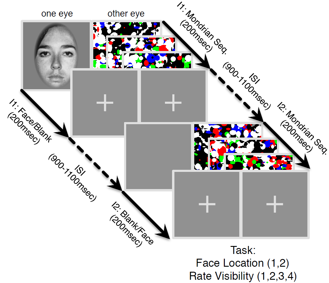
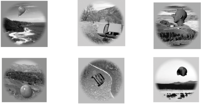
Figure | The continuous flash suppression paradigm used by the authors. A stimulus presented to one eye is rendered invisible by a sequence of Mondrian images presented to the other eye.
In a new paper, Haun, Oizumi, Kovach, Kawasaki, Oya, Howard, Adolphs, and Tsuchiya (pp2016) derive some interesting predictions from integrated information theory and test them with electrocorticography, measuring neuronal activity in human patients that have implanted subdural electrodes in their brains. The authors use the established psychophysical paradigms of continuous flash suppression and backward masking to render stimuli that are processed in cortex subjectively invisible and their representations, thus, unconscious.
The paper uses the previously described measure φ* of integrated information. This measure uses estimates of mutual information between past and present states of a set of measurement channels. The mutual information is estimated on the basis of multivariate Gaussian assumptions. Computing φ* involves estimating the effects of partitioning the set of channels, by modelling the partition distributions as independent (i.e. the joint distribution obtains as the product of the partitions’ distribution). φ* is the loss in system past-to-present predictability incurred by the least destructive partitioning.
The paper introduces the concept of the φ* pattern, the pattern of φ* estimates across subsets of components of the system (where electrodes pragmatically serve to define the components). The φ* pattern is hypothesized to reflect the compositional structure of the conscious percept.
Results suggest that stronger φ* values for certain sets of electrodes in the fusiform gyrus, which pick up on face-selective responses, are associated with conscious percepts of faces (as opposed to Mondrian images or visual noise). This association holds even across sets of trials, where the physical stimulus was identical and only the internal dynamics rendered the face representation conscious or unconscious. The authors argue that these results support IIT and suggest that the φ* pattern reflects information about the conscious percept.
Strengths
- The ideas in the paper are creative, provocative, and inspiring.
- The paper uses well-established psychophysical paradigms to control the contents of consciousness and disentangle conscious perception from stimulus representation.
- The φ* measure is well motivated by IIT and has been introduced in earlier work involving some of the authors – even if its relationship to consciousness is speculative.
Weaknesses
- The authors introduce the φ* pattern and hypothesize that it reflects the compositional structure of conscious content. However, theoretically, it is unclear why it should be that pattern across subsets of components, rather than simply the pattern across components that reflects the compositional structure of conscious content. Empirically, results are most parsimoniously summarised by saying that φ* tends to be larger when the content represented by the underlying neuronal population is conscious. The evidence for a reflection of the compositional structure of conscious content in the φ* pattern is weak.
- It is unclear how φ* is related to the overall activity in sets of neurons selective for the perceptual content in question (faces here). This leaves open the possibility that face selective neurons are simply more active when the face percept is conscious and this greater activity is associated with greater interactivity among the neurons, reflecting their structural connectivity.
- The finding that the alternative measures, state entropy H and (past-present) mutual information I, are less predictive of conscious percepts does not provide strong constraints on theory, because these measures are not particularly plausible to begin with and no compelling theoretical motivation is given for them.
- IIT suggests that integrated information across the entire brain supports consciousness. An unavoidable challenge for empirical studies, as the authors appropriately discuss, is the limitation of the φ* estimates to small sets of empirical measurements of brain activity.
Particular points the authors may wish to address in revision
(1) Are face-selective populations of neurons simply more active when a face is consciously perceived and φ* rises as an epiphenomenon of greater activity in the interconnected set of neurons?
It is left unclear whether the level of percept-specific neuronal activity provides a comparably good or better neural correlate of conscious content. The data presented have been analysed with more conventional activity-based pattern classification in Baroni et al. (pp2016) and results suggest that this also works. What if the substrate of consciousness is simply strong activity or activity in certain frequency bands and the φ* just happens to be a measure correlated with those simpler measures in a population of neurons? After all, we would expect an interconnected neuronal population to exhibit greater dynamic interactivity when it is strongly driven by a stimulus. The key challenge left unaddressed is to demonstrate that φ* cannot be reduced to this classical neuronal correlate of perceptual content. Do the two tend to be correlated? Can they be disentangled experimentally?
A compelling demonstration would be to show that φ* (or another IIT-motivated measure) captures variance in conscious content that is not explained by conventional decoding features. For example, two populations of neurons – one coding a face, the other a Mondrian – might be equally activated overall by a stimulus containing both a face and a Mondrian, but φ* computed for each population might enable us to predict the consciously perceived stimulus on a trial-by-trial basis.
(2) Does the φ* pattern reflect the conscious percept and its compositional structure?
A demonstration that the φ* pattern (across subsets) reflects the compositional structure of the content of consciousness would require an experiment eliciting a wider range of conscious percepts that are composed of a set of elements in different combinations.
The authors’ hypothesis would then have to be compared to a range of simpler hypotheses about the neural correlates of compositional conscious content (NC4) , including the following:
- the pattern of activity across content-selective neural sites
(rather than the across a subsets of sites) - the pattern of activity across subsets of sites
- the connectivity across content-selective neural sites (where connectivity could be measured by synchrony, coherence, Granger causality or any other measure of the relationship between two sites)
- the connectivity across content-selective neural subsets of sites
This list could be expanded indefinitely and could include a variety of IIT-inspired but distinct NC4s. There are many ideas that are similarly theoretically plausible, so empirical tests might be the best way forward.
In the discussion the authors argue that integrated information has greater a priori theoretical support than arbitrary alternative neural correlates of consciousness. There is some truth to that. However, the theoretical motivation, while plausible and and interesting, is not so uniquely compelling that it supports lowering the bar of empirical confirmation for IIT measures.
(3) Might the selection of channels by maximum φ* have introduced a bias to the analyses?
I understand that the selection was performed without using the conscious/unconscious trial labels. However, conscious percepts are likely to be associated with greater activity, and φ* might be confounded by greater activity. More generally, selection biases are often complicated, and without a compelling demonstration that there can be no selection bias, it is difficult to be confident. A simple way to rule out selection bias is to use independent data for selection and selective analysis.
– Nikolaus Kriegeskorte
Acknowledgement
I thank Kate Storrs for discussing integrated information theory with me.

 Figure 2: Shades of Bayes. The authors follow Kevin Murphy’s textbook in defining degrees of Bayesianity of inference, ranging from maximum likelihood estimation (top) to full Bayesian inference on parameters and hyperparameters (bottom). Above is my slightly modified version.