[I7R8]
Deep convolutional neural networks can label images with object categories at superhuman levels of accuracy. Whether they are as robust to noise and distortions as human vision, however, is an open question.
Geirhos, Janssen, Schütt, Rauber, Bethge, and Wichmann (pp2017) compared humans and deep convolutional neural networks in terms of their ability to recognize 16 object categories under different levels of noise and distortion. They report that human vision is substantially more robust to these modifications.
Psychophysical experiments were performed in a controlled lab environment. Human observers fixated a central square at the start of each trial. Each image was presented for 200 ms (3×3 degrees of visual angle), followed by a pink noise mask (1/f spectrum) of 200-ms duration. This type of masking is thought to minimize recurrent computations in the visual system. The authors, thus, stripped human vision of the option to scrutinize the image and focused the comparison on what human vision achieves through the feedforward sweep of processing (although some local recurrent signal flow likely still contributed). Observers then clicked on one of 16 icons to indicate the category of the stimulus.
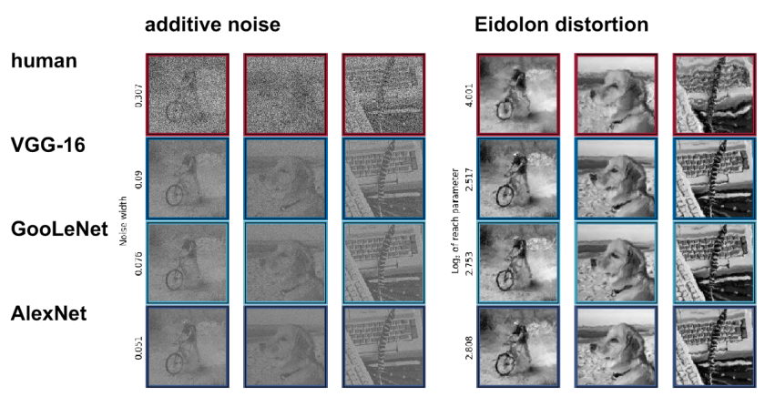
The figure below shows the levels of additive uniform noise (left) and local distortion (right) that were necessary to reduce the accuracy of each system to about 50% (classifying among 16 categories). Careful analyses across levels of noise and distortion show that the deep nets perform similarly to the human observers at low levels of noise or distortion. Both humans and deep nets approach chance level performance at very high levels of distortion. However, human performance degrades much more gracefully, beating deep nets when the image is compromised to an intermediate degree.
This is careful and important work that helps characterize how current models still fall short. The authors are making their substantial lab-acquired human behavioral data set openly available. This is great, because the data can be analyzed by other researchers in both brain science and computer science.
What the study does not quite deliver is an explanation of why the deep nets fall short. Is it something about the convolutional feedforward architecture that renders the models less robust? Does human vision employ normalization or adaptive filtering operations that enable it to “see through” the noise and distortion, e.g. by focusing on features less affected by the artefacts?
Humans have massive experience with noisy viewing conditions, such as those arising in bad weather. We also have much experience seeing things distorted, through water, or glass that is not perfectly plane. Moreover, peripheral vision may rely on summary-statistical descriptions that may be somewhat robust to the kinds of distortion used in this study.
To assess whether it is visual experience or something about the architecture that causes the networks to be less robust, I suggest that the networks be trained with noisy and/or distorted images. Data augmentation with noise and distortion may help deep nets learn more robust internal representations for vision.
Strengths
- Careful human psychophysical measurements of classification accuracy for 16 categories for a large set of stimuli (40K categorization trials).
- Detailed comparisons between human performance and performance of three popular deep net architectures (AlexNet, GoogLeNet, VGG-16).
- Substantial behavioral data set shared with the community.
Weaknesses
- Network architectures not trained with noise and distortion rendering ambiguous whether the deep nets’ lack of robustness is due to architecture or training.
- Data are not used to evaluate the three models overall in terms of their ability to capture patterns of confusions.
- Human-machine comparisons focus on overall accuracy under noise and distortion, and on category-level confusions, rather than the processing of particular images.
Suggestions for improvements
(1) Train deep nets with noise and distortion. Humans experience noise and distortions as part of their visual world. Would the networks perform better if they were trained with noisy and distorted images? The authors could train the networks (or at least VGG-16) with some image set (nonoverlapping with the images used in the psychophysics) and augment the training set with noisy and distorted variants. This would help clarify to what extent training can improve robustness and to what extent the architecture is the limiting factor.
(2) Evaluate each model’s overall ability to predict human patterns of confusions. The confusion matrix analyses shed some light on the differences between humans and models. However, it would be good to assess which model’s confusions are most similar to the humans overall. To this end one could consider the offdiagonal elements of the confusion matrix (to render the analysis complementary to the analyses of overall accuracy) and statistically compare the models in terms of their ability to explain patterns of confusions. The offdiagonal entries only could be compared by correlation (or 0-fixed correlation).
Minor comments
(1) “adversarial examples have cast some doubt on the idea of broad-ranging manlike DNN behavior. For any given image it is possible to perturb it minimally in a principled way such that DNNs mis-classify it as belonging to an arbitrary other category (Szegedy et al., 2014). This slightly modified image is then called an adversarial example, and the manipulation is imperceptible to human observers (Szegedy et al., 2014).”
This point is made frequently, although it is not compelling. Any learner uses an inductive bias to infer a model from data. In general, combining the prior (inductive bias) and the data will not yield perfect decision boundaries. An omniscient adversary can always place an example in the misrepresented region of the input space. Adversarial examples are therefore a completely expected phenomenon for any learning algorithm, whether biological or artificial. The misrepresented volume may have infinitesimal probability mass under natural conditions. A visual system could therefore perform perfectly in the real world — until confronted with an omniscient adversary that backpropagates through its brain to fool it. No one knows if adversarial examples can also be constructed for human brains. If so, they might similarly require only slight modifications imperceptible to other observers.
The bigger point that neural networks fall short of human vision in terms of their robustness is almost certainly true, of course. To make that point on the basis of adversarial examples, however, would requires considering the literature on black-box attacks that do not rely on omniscient knowledge of the system to be fooled or its training set. It would also require applying these much less efficient methods symmetrically to human subjects.
(2) “One might argue that human observers, through experience and evolution, were exposed to some image distortions (e.g. fog or snow) and therefore have an advantage over current DNNs. However, an extensive exposure to eidolon-type distortions seems exceedingly unlikely. And yet, human observers were considerably better at recognising eidolon-distorted objects, largely unaffected by the different perceptual appearance for different eidolon parameter combinations (reach, coherence). This indicates that the representations learned by the human visual system go beyond being trained on certain distortions as they generalise towards previously unseen distortions. We believe that achieving such robust representations that generalise towards novel distortions are the key to achieve robust deep neural network performance, as the number of possible distortions is literally unlimited.”
This is not a very compelling argument because the space of “previously unseen distortions” hasn’t been richly explored here. Moreover, the Eidolon-distortions are in fact motivated by the idea that they retain information similar to that retained by peripheral vision. They, thus, discard information that the human visual system is well trained to do without in the periphery.
(3) On the calculation of DNNs’ accuracies for the 16 categories: “Since all investigated DNNs, when shown an image, output classification predictions for all 1,000 ImageNet categories, we disregarded all predictions for categories that were not mapped to any of the 16 entry-level categories. Amongst the remaining categories, the entry-level category corresponding to the ImageNet category with the highest probability (top-1) was selected as the network’s response.”
It would seem to make more sense to add up the probabilities of the ImageNet categories corresponding to each of the 16 entry-level categories and use the resulting 16 totals to pick the predicted basic-level category. Alternatively, one may train a new softmax layer with 16 outputs. Please clarify which method was used and how it relates to the other methods.
–Nikolaus Kriegeskorte
Thanks to Tal Golan for sharing his comments on this paper with me.


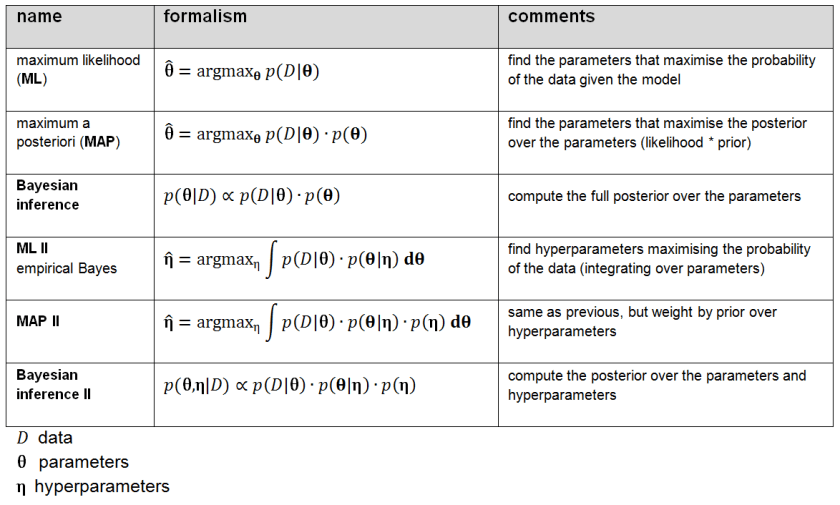 Figure 2: Shades of Bayes. The authors follow Kevin Murphy’s textbook in defining degrees of Bayesianity of inference, ranging from maximum likelihood estimation (top) to full Bayesian inference on parameters and hyperparameters (bottom). Above is my slightly modified version.